DSATools™ TSAT

Introduction

The DSATools™ TSAT Node performs dynamic study simulations which are powered by Transient Security Assessment Tool (TSAT), a 3rd party power systems software developed by Powertech Labs.

This Node is typically used for the following:

Completing dynamic studies (e.g. validating Generator Performance Standards).
Benchmarking plant models (e.g. comparing the performance of user defined and/or generic plant models).

info

Check our system requirements page for information on which TSAT versions are currently supported.

User inputs

Select model

Model

Defines the input directory and file name of the TSAT case file (.tsa). This file:

Must have a Base Scenario; and
This Base Scenario contain the file name(s) of any required dynamic data (.dat) file(s) for your generating system.

A valid power flow result is also required. If the Use model from linked PSAT or PSS®E Static Node option is not selected, you must provide a power flow result linked in your .tsa case file.

If the Use model from linked PSAT or PSS®E Static Node option is selected, the gridmo Engine will use the output of a connected PSS®E Static or PSAT Node as the power flow result to initialize TSAT (the power flow result in your .tsa case file will be ignored).

Example:

sunny-solar-farm\SMIB.tsa

note

File paths are relative to the Engine's 'inputs' directory, as defined by the Engine configuration parameter dirs.inputs. For example, if dirs.inputs was set as C:\Users\johnsmith\gridmo\Inputs\:

Absolute file path	Relative file path (required by gridmo)
C:\Users\johnsmith\gridmo\Inputs\sunny-solar-farm\SMIB.tsa	sunny-solar-farm\SMIB.tsa

The gridmo Engine will copy all files, excluding some unnecessary file types (e.g. .pdf) to a temporary processing directory, including subfolders located where the specified .tsa case file is located. You don't need to specify the path to each additional file defined in the .tsa files, e.g. .dat files - the gridmo Engine will copy these automatically.

danger

All scenarios except for the Base Scenario in the .tsa file will be ignored. The gridmo Engine uses the Base Scenario to create the tests specified in the web-app.

Define simulation

Simulation time

Defines the duration of the dynamic study in seconds.

Example: Run a 30 second dynamic simulation.

note

The minimum simulation time is 0.1 seconds.

info

🔢 Supports mathematical operations.

info

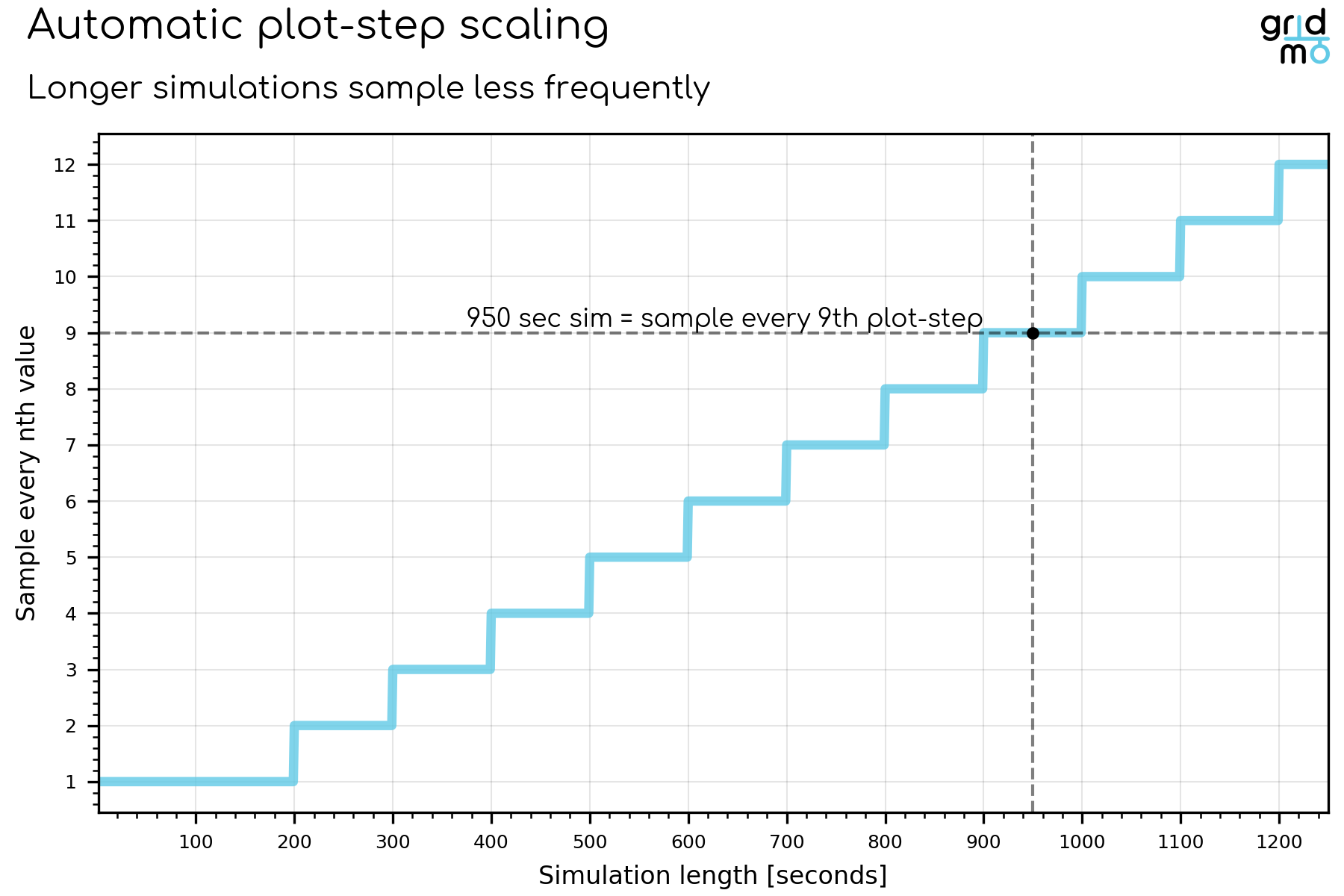
The resolution of the output data (plot step) is automatically reduced if the simulation time is above 200 seconds.

This is to reduce size of output files and temporary files generated during the simulation.

For example, if gridmo is running a 950 second long simulation, gridmo will set TSAT's plot step so that one channel data point is exported for every nine time steps, based on the below relationship.

graph on the horizontal axis is simulation time and vertical axis is plot step scaling factor

Control Thévenin equivalent source

These controls allow you to define the behaviour of the grid.

You can control:

Voltage [p.u.]; or
Frequency [Hz]; or
Angle [degrees]; or

note

TSAT does not support controlling both frequency and angle playback simultaneously.

Voltage

Defines the Thévenin bus voltage throughout the dynamic simulation. Enter a series of time [s], voltage [p.u.] pairs. The voltage is linearly interpolated between points. There are two methods for specifying the voltage - absolute and relative.

note

If your DSATools™ TSAT study uses a case file from a linked PSAT or PSSE Static Node, it is often convenient to specify the voltage using the relative method, since it will utilize the Thévenin bus voltage solution from that specific case.

Specifying absolute voltage

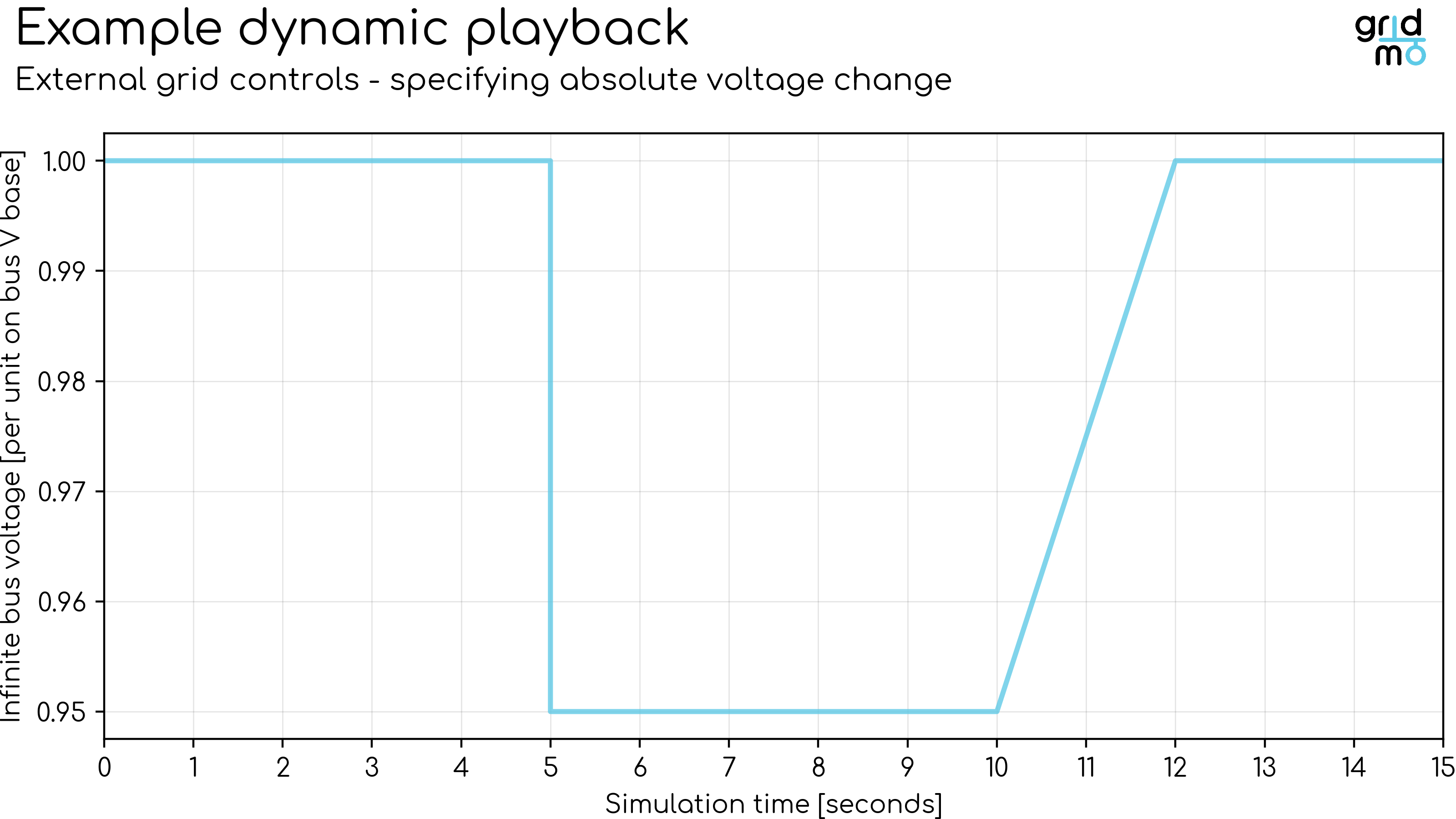
Defines the Thévenin bus voltage throughout the dynamic simulation by specifying absolute voltage [p.u.].

Example: Perform a 15 second dynamic simulation. At 5 seconds, step the voltage from 1.00 [p.u.] to 0.95 [p.u.] in a single rapid step. At 10 seconds, ramp the voltage back up to 1.00 [p.u.] over 2 seconds.

Example

0,      1.00
4.9999, 1.00
5,      0.95
10,     0.95
12,     1.00
15,     1.00

Plot

Specifying relative voltage

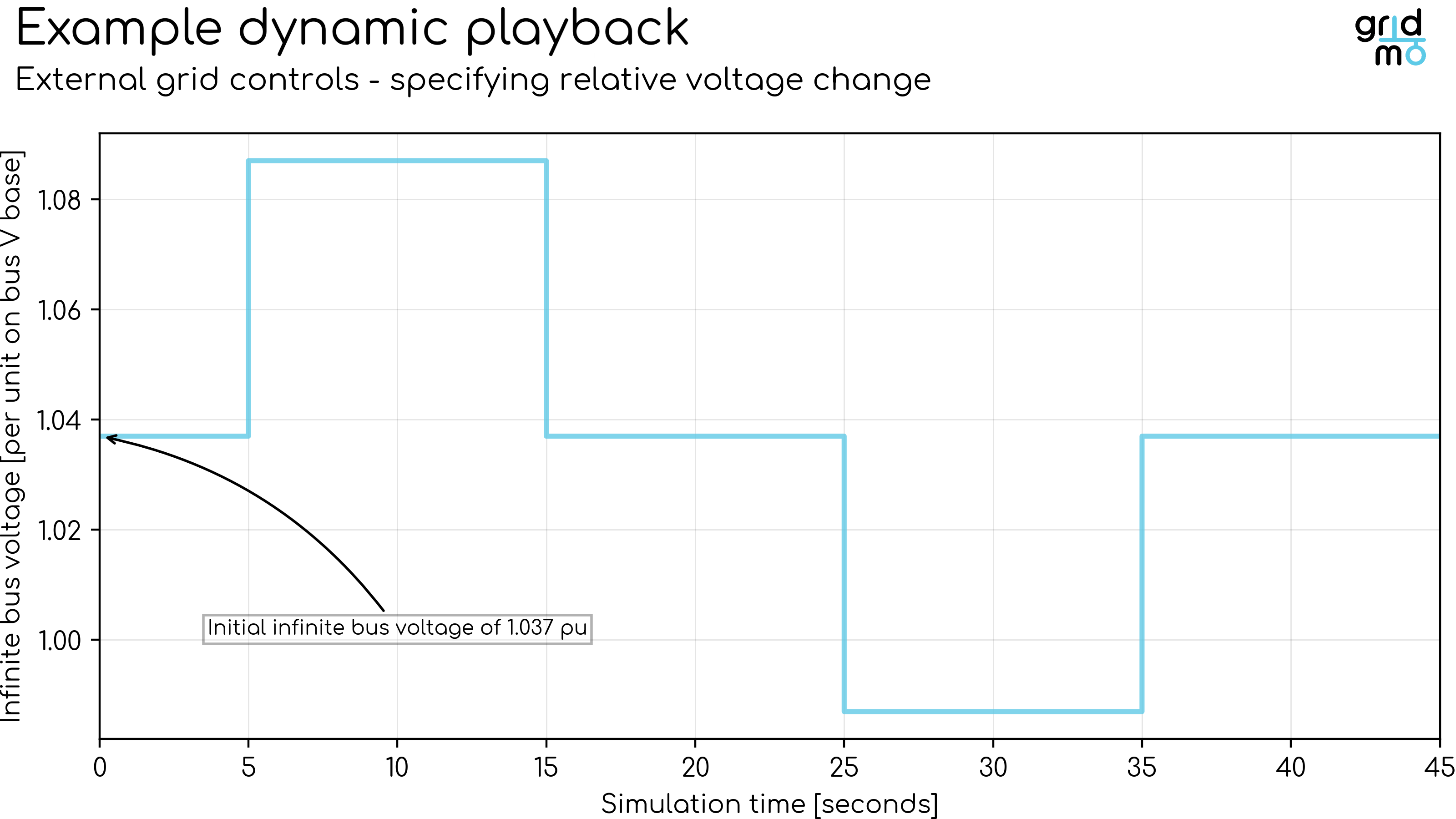
Defines the Thévenin bus voltage throughout the dynamic simulation by specifying relative voltage [p.u.]. The voltage change is relative to the voltage of the Thévenin bus voltage at the start of the dynamic simulation.

Example: Perform a 45 second dynamic simulation. At 5 seconds, step the voltage up 0.05 per unit [p.u.] in a single rapid step. At 15 seconds, step the voltage down to its initial value in a single rapid step. At 25 seconds, step the voltage down 0.05 per unit [p.u.] in a single rapid step. At 35 seconds, step the voltage up to its initial value in a single rapid step.

Example

0,      0 pu
4.999,  0 pu
5,      +0.05 pu
14.999, +0.05 pu
15,     0 pu
24.999, 0 pu
25,     -0.05 pu
34.999, -0.05 pu
35,     0 pu
45,     0 pu

Plot

Frequency

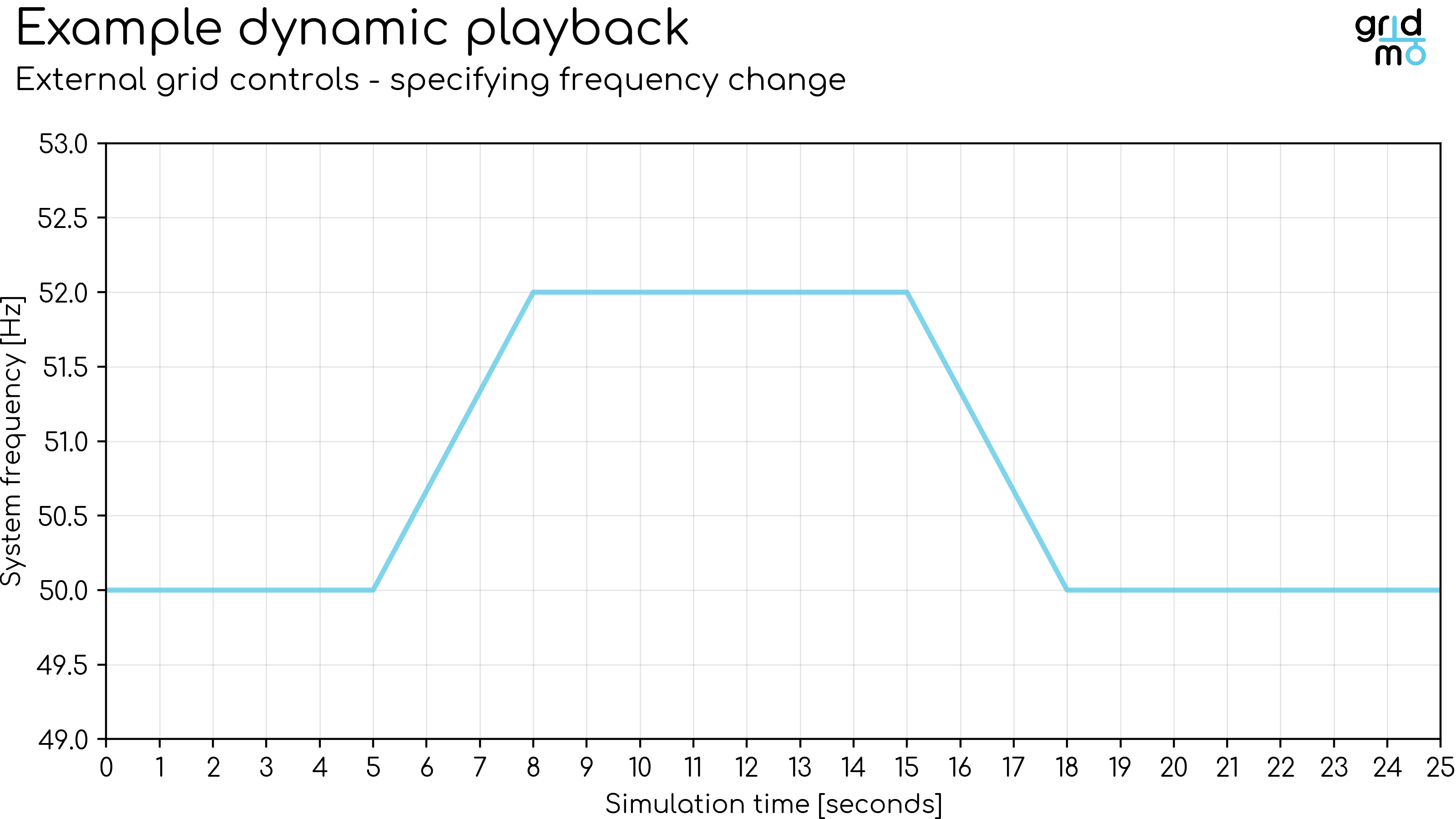
Defines the Thévenin bus frequency throughout the dynamic simulation. Enter a series of time [s], frequency [Hz] pairs. The frequency is linearly interpolated between points.

Example: Perform a 25 second dynamic simulation. At 5 seconds, ramp the frequency up from 50.0 [Hz] to 52.0 [Hz] over 3 seconds. At 15 seconds, ramp the frequency back down to 50.0 [Hz] over 3 seconds.

Example

Plot

Angle

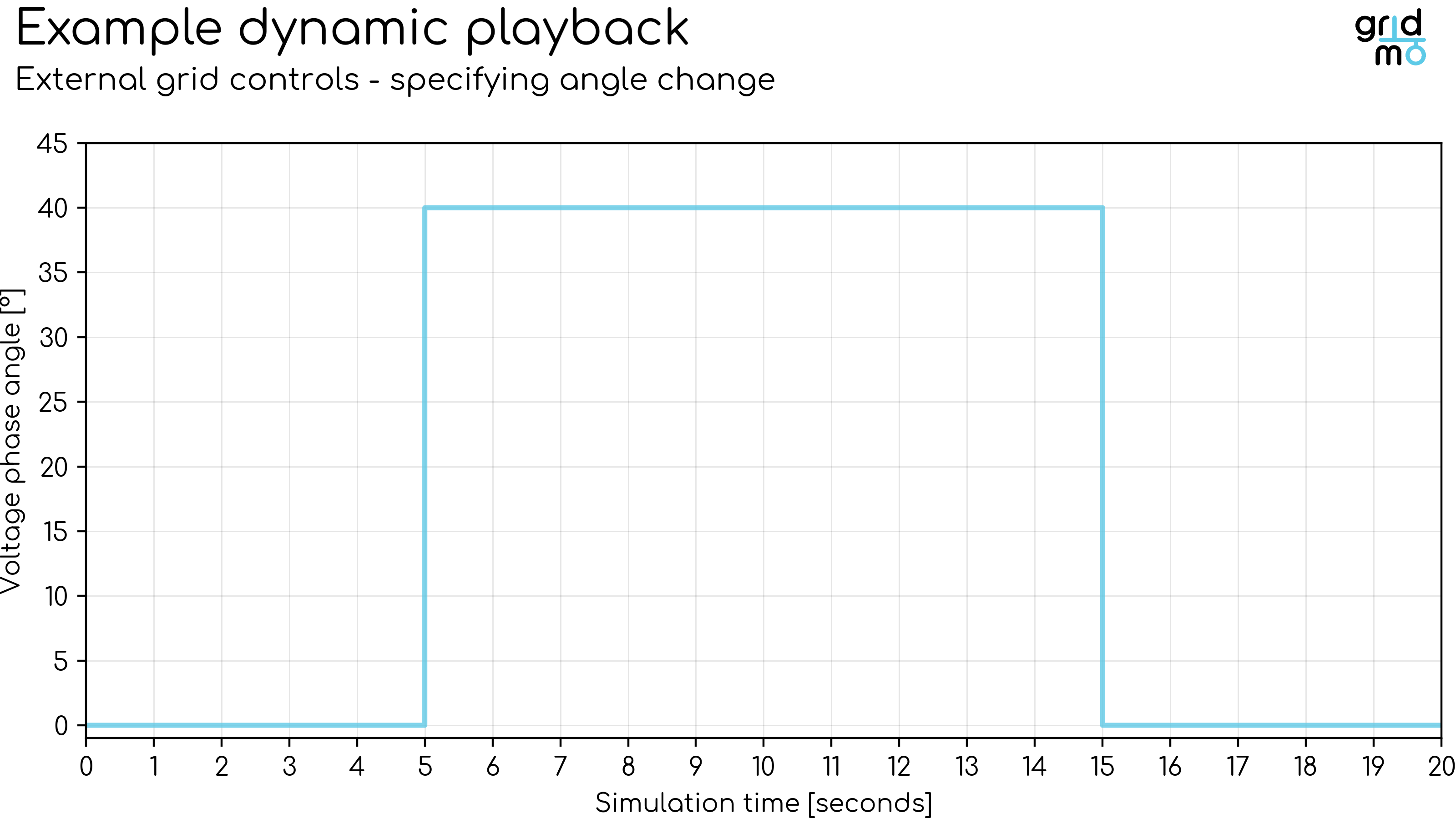
Defines the Thévenin bus voltage phase angle throughout the dynamic simulation. Enter a series of time [s], angle [degrees] pairs. The voltage phase angle is not linearly interpolated between points - instead the angle is set to the absolute value at the time specified. The voltage phase angle values specified are relative to the initial angle at the Thévenin bus - which is typically 0° for SMIB studies.

caution

Voltage phase angle changes are instantaneous. Ramps are not supported.

Example: Perform a 20 second dynamic simulation. At 5 seconds, step the voltage phase angle from 0° to 40°. At 15 seconds, step the voltage phase angle back to 0°.

Example

0,  0
5,  40
15,  0

Plot

Actions

Defines the Commands which configure the dynamic simulation.

Supported Commands:

Applied BEFORE TSAT is opened:
- SETFILE: Sets the value of a parameter in an external text or configuration file.
Applied DURING the simulation:
- SET: Sets the status or value of a network element (e.g. bus, line, generator).
- CONTROL: Controls a network element.
- SIMPLEFAULT: Applies a simple power system fault.

caution

If you specify the value of the AT= argument beyond the simulation duration (e.g. simulation duration is 20 [s] and AT=25), the Command will not be applied and a warning will be raised.

Define outputs

Outputs

Defines the output channels of the dynamic simulation. The output channels defined here may be used later for plotting and/or further analysis.

Supported Commands:

OUTPUT: Outputs a network element's dynamic simulation values as an Internode Variable.

info

OUTPUT Commands do not require the AT= argument because dynamic simulation values are recorded for the entire simulation.

Description

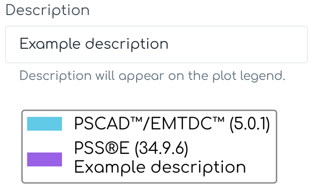
Defines a short description of the dynamic simulation. This description will appear in the legend of any plot of the data generated by this Node.

Example:

Description here!

example from a Plot Node PDF output showing how the 'Description here!' text is added

Advanced

TSAT version

Defines the TSAT version used for the Node. Defaults to Engine configuration.

See here for details on how to specify partial versions.

Distance factor

Defines the distance from the connection point at which disturbances are applied. Allowable values are between 0 and 1, where d=1 applies disturbances at the connection point. The image below shows a Thévenin equivalent of the grid as used in SMIB studies, commonly referred to as the 'infinite source', whereby:

V_thev: Thévenin equivalent voltage source.
Z_thev: Thévenin equivalent impedance.
Z_f: Disturbance impedance.
d: Distance factor.
V_poc: Connection point voltage prior to any disturbance.

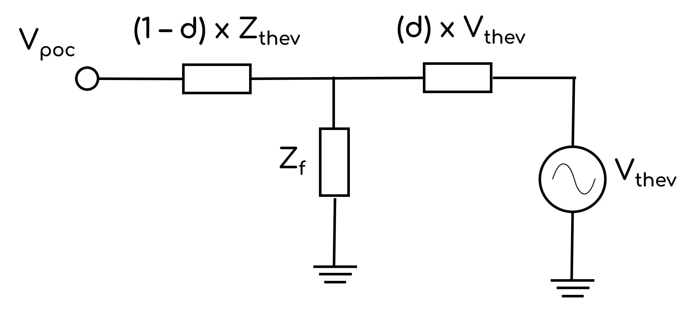
Distance factor will apply to all relevant Commands in the Node such as:

SIMPLEFAULT

Advanced Parameters

Advanced Parameters allow users to configure test details which are not commonly used. Advanced Parameters are often specific to each Node type.

Each line represents a new Advanced Parameter and is entered as a=b format, where a is the name of the Parameter and b is the corresponding value. All Advanced Parameters are set to their default values if they are not included in the Advanced Parameters field.

Example: Set Advanced Parameter, sample.parameter to a value of 5.

sample.parameter=5

API Reference

This section details the Commands and Advanced Parameters specific to the Node.

tip

Lines are defined using the following syntax: from->to#id.

When completing SMIB studies, we recommend the line points in the direction towards the bulk electrical grid (the to bus being closer to your Thévenin source) for easy interpretation of results.

`SETFILE` Command

SETFILE, FILENAME=, PARAM/NUMBER=, VAL=

Before TSAT is opened, modifies the FILENAME= external file by finding the PARAM= setting and updating its value to VAL=. Supports basic text formats with delimiters such as comma, space, tab and equals.

Arguments:

SETFILE
FILENAME (str): Defines the relative input directory and file name of the text file to be modified.
PARAM or NUMBER:
- PARAM (str): Parameter name. If the configuration file has section titles in square brackets, the PARAM= field should be in the format [SectionTitle].ParameterName.
- NUMBER (int): Line number.
VAL 🔢 (float or int or str): Value. If PARAM= is used, VAL is the parameter value. If NUMBER= is used, VAL is the value of the entire line in the file.

note

The text file specified by the FILENAME= field is only modified in the copy of the model in the Engine's working directory. It is not modified in the Engine's inputs folder.

tip

If you need to modify a settings file with format like the below, you can still use the SETFILE command.

You need to set the PARAM= field to [SectionTitle].ParameterName (use the actual values from your settings file) and set the VAL= field to the new value.

[SectionTitle]
ParameterName=0.5

Example: Before TSAT has opened, modify the file windy_wind_farm\ppc_settings.dyr to put the plant in power factor control mode. The .dyr file has been formatted such that the required ICON value is on its own line inside the file on line 17. The parameter PPC_Q_ControlMode needs to be set to a value of 200.

SETFILE, FILENAME=windy_wind_farm\ppc_settings.dyr, NUMBER=17, VAL=200

`SET` Command

Set bus

SET, BUS=, [BUS=], AT=, STATUS=

Sets the status of a bus.

Arguments:

SET
BUS (int): Bus number.
BUS (int)[Optional]: Additional bus numbers.
AT 🔢 (float): Time at which the Command is applied during the dynamic simulation [s].
STATUS (str): Bus status. Options:
- STATUS=OUT: Status is out of service.

note

TSAT currently only allows a bus to be switched out of service. It cannot be switched in during a simulation.

Example: At 5 seconds, set bus 100 out of service.

SET, BUS=100, AT=5, STATUS=OUT

Set line

SET, LINE=, [LINE=, AT=, STATUS=, SCR=, XR=]

Sets the status and impedance of a line.

Arguments:

SET
LINE (pas): Line definition. Lines are defined using the following syntax: from->to#id.
LINE (pas)[Optional]: Additional line definitions (only if using STATUS=, SCR= and XR= arguments only support one line)
AT 🔢 (float): Time at which the Command is applied during the dynamic simulation [s].
STATUS (str)[Optional]: Line status. Options:
- STATUS=IN: Status is in-service.
- STATUS=OUT: Status is out of service.
SCR (float)[Optional] Set the Short Circuit Ratio and X/R Ratio::
- SCR=X (where X is a number): Sets the impedance of the given line to the equivalent Thévenin impedance based on the Project's rated active power [MW], the line voltage and the specified SCR and X/R ratio.
- SCR=INF: Sets the impedance of the given line to the minimum cross-software stable impedance. XR= Argument is ignored and X/R ratio is forced to infinite.
XR 🔢 (float)[Optional]: The reactance to resistance ratio to apply to the specified line.

note

SCR and XR Arguments must be used together. These Arguments are typically only used in SMIB studies and are used to calculate the Thévenin equivalent source impedance of the infinite generator.

Example: At 14.7 seconds, set the impedance of the line from bus 800 to bus 900 which has an ID of 1. The line impedance should represent the system Thévenin equivalent impedance for an SCR of 3 and X/R ratio of 2.

SET, LINE=800->900#1, AT=14.7, STATUS=IN, SCR=3, XR=2

`CONTROL` Command

`CONTROL_UDM` Change UDM Block

CONTROL_UDM, GEN/LINE=, [GEN/LINE=], TYPE=, BLOCK=, [VAL_FUNCTION=], AT=, VAL/RELVAL=

Issues a relative reference command to the specified generator(s) at the specified time in the simulation. The gridmo Engine controls the generator using a Change UDM Block TSAT command.

Arguments

CONTROL_UDM
GEN or LINE:
- GEN (pas): Generator definition. Generators are defined using the following syntax: bus#id.
- GEN (pas)[Optional]: Additional generator definitions. Generators are defined using the following syntax: bus#id.
- LINE (pas): Line definition. Lines are defined using the following syntax: from->to#id.
- LINE (pas)[Optional]: Additional line definition. Lines are defined using the following syntax: from->to#id.
  TYPE (str): User defined model type. Options:
  TYPE=EXCUDM: Exciter UDM
  TYPE=PSSUDM: Power system stabilizer UDM
  TYPE=UELUDM: Underexcitation limiter UDM
  TYPE=OELUDM: Overexcitation limiter UDM
  TYPE=GOVUDM: Prime mover and speed governing UDM
  TYPE=SHCUDM: Shunt compensator UDM
  TYPE=WTGUDM: Renewable generator UDM
  TYPE=SECUDM: Series compensator UDM
  TYPE=SERPAR
  TYPE=SERVMR
  TYPE=SPSBUS: System protection scheme associated with a bus
  TYPE=SPSGEN: System protection scheme associated with a generator
  TYPE=SPSBRN: System protection scheme associated with a branch
  TYPE=SPSUDM: System protection scheme
  TYPE=WGNUDM: Generator/Convertor model in modularized renewable generator
  TYPE=WPQUDM: Electrical Controller model in modularized renewable generator
  TYPE=WTQUDM: Torque Controller model in modularized renewable generator
  TYPE=WMCUDM: Mechanical system model in modularized renewable generator
  TYPE=WPTUDM: Plant controller model in modularized renewable generator
  TYPE=SUPBUS
  TYPE=SUPUDM
  TYPE=SWSUDM
BLOCK (str): User defined model block.
VAL_FUNCTION 🔢 (str)[Optional]: Function applied to RELVAL. For example, VAL_FUNCTION=2*VAL+1. Click here for more information on VAL_FUNCTION syntax and supported functions.
AT 🔢 (float): Time at which the Command is applied during the dynamic simulation [s].
VAL or RELVAL:
- VAL 🔢 (float): New value, expressed absolutely (i.e. Action = SET).
- RELVAL 🔢 (float): Relative change to value value, expressed relatively (i.e. Action = DELTA).

Examples

Assuming my generator reactive power reference is in MVAr, apply a relative reactive power reference change of -10 MVAr at 5 seconds for my generator with ID 1 at bus 100 which uses a UDM type of WPTUDM and a block parameter QAUX.

CONTROL_UDM, GEN=100#1, TYPE=WPTUDM, BLOCK=QAUX, AT=5, RELVAL=-10

`CONTROL_RG` Change renewable generator reference

CONTROL_RG, GEN=, [GEN=], TYPE=, [VAL_FUNCTION=], AT=, RELVAL=

Issues a relative reference command to the specified generator(s) at the specified time in the simulation. The gridmo Engine controls the generator using a Change renewable generator reference TSAT command.

Arguments

CONTROL_RG
GEN (pas): Generator definition. Generators are defined using the following syntax: bus#id.
GEN (pas)[Optional]: Additional generator definitions. Generators are defined using the following syntax: bus#id.
TYPE (str): Type of reference signal. Options:
- TYPE=PG: Active power.
- TYPE=QG: Reactive power.
- TYPE=VT: Voltage.
- TYPE=PF: Power factor.
VAL_FUNCTION 🔢 (str)[Optional]: Function applied to RELVAL. For example, VAL_FUNCTION=2*VAL+1. Click here for more information on VAL_FUNCTION syntax and supported functions.
AT 🔢 (float): Time at which the Command is applied during the dynamic simulation [s].
RELVAL 🔢 (float): Relative change to active power setpoint [unit depends on model under control].

danger

Currently, the gridmo Engine can only apply relative reference changes.

Examples

Assuming my generator reactive power reference is in MVAr, apply a relative reactive power reference change of -10 MVAr at 5 seconds for my generator with ID 1 at bus 100.

CONTROL_RG, GEN=100#1, TYPE=QG, AT=5, RELVAL=-10

`CONTROL_GREF` Change governor reference

CONTROL_GREF, GEN=, [GEN=], [VAL_FUNCTION=], AT=, RELVAL=

Issues a relative governor (speed) reference command to the specified generator(s) at the specified time in the simulation. The gridmo Engine controls the generator using a Change governor reference TSAT command.

Arguments:

CONTROL_GREF
GEN (pas): Generator definition. Generators are defined using the following syntax: bus#id.
GEN (pas)[Optional]: Additional generator definitions. Generators are defined using the following syntax: bus#id.
VAL_FUNCTION 🔢 (str)[Optional]: Function applied to RELVAL. For example, VAL_FUNCTION=2*VAL+1. Click here for more information on VAL_FUNCTION syntax and supported functions.
AT 🔢 (float): Time at which the Command is applied during the dynamic simulation [s].
RELVAL 🔢 (float): Relative change to power factor setpoint [unit depends on model under control].

danger

Currently, the gridmo Engine can only apply relative reference changes.

Example: At 5 seconds, change the governor reference of the generator model at bus 500 with an ID of 2. Change governor speed by +0.02 [p.u.] relative to the current speed/value.

CONTROL_GREF, GEN=500#2, AT=5, RELVAL=0.02

`CONTROL_VREF` Change AVR reference

CONTROL_VREF, GEN=, [GEN=], [VAL_FUNCTION=], AT=, RELVAL=

Issues a relative voltage (AVR) reference command to the specified generator(s) at the specified time in the simulation. The gridmo Engine controls the generator using a Change AVR reference TSAT command.

Arguments:

CONTROL_VREF
GEN (pas): Generator definition. Generators are defined using the following syntax: bus#id.
GEN (pas)[Optional]: Additional generator definitions. Generators are defined using the following syntax: bus#id.
VAL_FUNCTION 🔢 (str)[Optional]: Function applied to RELVAL. For example, VAL_FUNCTION=2*RELVAL+1. Click here for more information on VAL_FUNCTION syntax and supported functions.
AT 🔢 (float): Time at which the Command is applied during the dynamic simulation [s].
RELVAL 🔢 (float): Relative change to power factor setpoint [unit depends on model under control].

danger

Currently, the gridmo Engine can only apply relative reference changes.

Example: At 5 seconds, change the voltage reference of the generator model at bus 500 with an ID of 2. Change voltage reference by +0.04 [p.u.] relative to the current value.

CONTROL_VREF, GEN=500#2, AT=5, RELVAL=0.04

`SIMPLEFAULT` Command

SIMPLEFAULT, LINE=, AT=, DURATION=, [FZ=0, XR=3]

Applies a simple three phase fault at a line. The line remains in-service during and after the fault is cleared. Fault impedance is specified in ohms.

Arguments:

SIMPLEFAULT
LINE (pas): Line definition. Lines are defined using the following syntax: from->to#id. The fault is applied at the from bus.
AT 🔢 (float): Time at which the fault is applied during the dynamic simulation [s].
DURATION (float): Fault duration [ms]. When the duration has expired, the fault is removed and the line will remain in service.
FZ [Optional]: Fault impedance in ohms [Ω]. Default value is 0 Ω (i.e. bolted fault).
XR 🔢 (float)[Optional]: Reactance to resistance ratio of the fault. Default value is 3.

danger

Currently, SIMPLEFAULT only supports three phase faults.

Example:

At 5 seconds, apply a three phase fault at the connection point bus of the SMIB model (where the from bus 500 is the connection point and the to bus 999 is the slack bus).
Fault duration is 430 ms.
Fault impedance is 10 Ω.
X/R ratio of the fault is 3.

SIMPLEFAULT, LINE=500->999#1, AT=5, DURATION=430, FZ=10, XR=3 

`OUTPUT` Command

caution

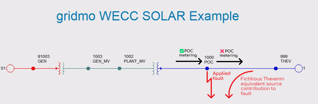
By default when completing SMIB studies, the Thevenin equivalent voltage source and impedance should not be used for POC metering in OUTPUT Commands or in generating system dynamics model data file (i.e. .dyr files).

During certain SMIB events (e.g. faults, consideration of distance factor, voltage phase angle playback), there will be fictitious Thevenin equivalent source contribution or we will need to break the Thevenin equivalent impedance line into multiple parts to complete the event. See the image below considering the example of applying a fault using SIMPLEFAULT; and

For clarity:

✅ Example of recommended POC metering:

OUTPUT, TX=1002->1000#1, METERBUS=1000, VAL=P, NAME=i_ch_poc_p
OUTPUT, TX=1002->1000#1, METERBUS=1000, VAL=Q, NAME=i_ch_poc_q

❌ Example of incorrect POC metering:

OUTPUT, LINE=1000->999#1, VAL=P, NAME=i_ch_poc_p
OUTPUT, LINE=1000->999#1, VAL=Q, NAME=i_ch_poc_q

Output bus variable

OUTPUT, BUS=, VAL=, [VAL_FUNCTION=], NAME=, [PLOT_STYLE=SOLID, DISPLAY_ONLY=NO, LEGEND=]

Outputs a variable from a bus.

Arguments:

OUTPUT
BUS (int): Bus number.
VAL (str): Bus value. Options:
- VAL=V: Voltage [p.u.].
- VAL=F: Frequency [Hz].
- VAL=ANGLE: Angle [degrees]. Angles are releative to the Thevenin source generator, or can be specified by using the angles.relative.to.generator Advanced Parameter.
VAL_FUNCTION 🔢 (str)[Optional]: Function applied to the output value(s). For example, VAL_FUNCTION=2*VAL+1. Click here for more information on VAL_FUNCTION syntax and supported functions.
NAME (str): Output name. Output names must be unique within a Node.
PLOT_STYLE (str)[Optional]: How this output channel should be plotted on connected Plot Nodes. Defaults to TYPE=SOLID. Options:
- TYPE=SOLID: A solid line.
- TYPE=DASHED: A dashed line.
DISPLAY_ONLY (bool)[Optional]: If YES, calculations (such as SETTLING_TIME) will not be performed using this output channel. Default value is NO.
LEGEND (str)[Optional]: Subplot legend name. Default value is no legend name.

Example: Output the voltage [p.u] at bus 100, name this output "i_poc_v".

OUTPUT, BUS=100, VAL=V, NAME=i_poc_v

Output line variable

OUTPUT, LINE=, [METERBUS=], VAL=, [PBASE=, QBASE=, SBASE=, VAL_FUNCTION=], NAME=, [PLOT_STYLE=SOLID, DISPLAY_ONLY=NO, LEGEND=]

Outputs a variable from a line.

Arguments:

OUTPUT
LINE (pas): Line definition. Lines are defined using the following syntax: from->to#id. Values are given at the 'from-side' of the line.
METERBUS (int)[Optional]: Bus number which is the metering point for the LINE= line. Default value is the 'from' bus number as per the LINE= argument.
VAL (str): Line value. Options:
- VAL=P: Active power [MW].
- VAL=Q: Reactive power [MVAr].
- VAL=S: Apparent power [MVA].
- VAL=PF: Power factor [unitless] (positive power factor corresponds to active power travelling towards the to bus from the from bus). Click here for details on how gridmo calculates power factor.
- VAL=I: Current [p.u.] on SBASE, where I [p.u.] = S [MVA] / (V [p.u.] * SBASE [MVA]).
- VAL=ID: Active current [p.u.] on PBASE; where ID [p.u.] = P [MW] / (V [p.u.] * PBASE [MW]).
- VAL=IQ: Reactive current [p.u.] on QBASE; where IQ [p.u.] = Q [MVAr] / (V [p.u.] * QBASE [MVAr]).
PBASE 🔢 (float)[Optional]: MW base used for Id calculation [MW]. Only required if VAL=ID .
QBASE 🔢 (float)[Optional]: MVAr base used for Iq calculation [MVAr]. Only required if VAL=IQ.
SBASE 🔢 (float)[Optional]: MVA base used for I calculation [MVA]. Only required if VAL=I.
VAL_FUNCTION 🔢 (str)[Optional]: Function applied to the output value(s). For example, VAL_FUNCTION=2*VAL+1. Click here for more information on VAL_FUNCTION syntax and supported functions.
NAME (str): Output name. Output names must be unique within a Node.
PLOT_STYLE (str)[Optional]: How this output channel should be plotted on connected Plot Nodes. Defaults to TYPE=SOLID. Options:
- TYPE=SOLID: A solid line.
- TYPE=DASHED: A dashed line.
DISPLAY_ONLY (bool)[Optional]: If YES, calculations (such as SETTLING_TIME) will not be performed using this output channel. Default value is NO.
LEGEND (str)[Optional]: Subplot legend name. Default value is no legend name.

Example: Output the active power flowing through the line from bus 100 to bus 200 (measured at the 'from-side' of the line) which has an ID of 1. Name this output "i_poc_p".

OUTPUT, LINE=100->200#1, VAL=P, NAME=i_poc_p

Example: Output the active power flowing through the line from bus 100 to bus 200 (measured at the 'to-side' of the line) which has an ID of 1. Name this output "i_poc_p_farend".

OUTPUT, LINE=100->200#1, METERBUS=200, VAL=P, NAME=i_poc_p_farend

Example: Output the reactive current flowing through the line from bus 100 to bus 200 (measured at the 'from-side' of the line) which has an ID of 1. The QBASE used in the reactive current calculation is 15 MVAr. Name this output i_poc_iq.

OUTPUT, LINE=100->200#1, VAL=IQ, QBASE=15, NAME=i_poc_iq

Output transformer variable

OUTPUT, TX=, [METERBUS=], VAL=, [PBASE=, QBASE=, SBASE=, VAL_FUNCTION=], NAME=, [PLOT_STYLE=SOLID, DISPLAY_ONLY=NO, LEGEND=]

Outputs a variable from a transformer.

Arguments:

OUTPUT
TX (pas): Transformer definition. Transformers are defined using the following syntax: bus1->bus2#id.
METERBUS (int)[Optional]: Bus number which is the metering point for the TX= line. Default value is the 'from' bus number as per the TX= argument. Not supported for three-winding transformers.
VAL (str): Transformer value. Options:
- VAL=P: Active power [MW].
- VAL=Q: Reactive power [MVAr].
- VAL=S: Apparent power [MVA].
- VAL=PF: Power factor [unitless] (positive power factor corresponds to active power travelling towards the to bus from the from bus). Click here for details on how gridmo calculates power factor.
- VAL=I: Current [p.u.] on SBASE, where I [p.u.] = S [MVA] / (V [p.u.] * SBASE [MVA]).
- VAL=ID: Active current [p.u.] on PBASE; where ID [p.u.] = P [MW] / (V [p.u.] * PBASE [MW]).
- VAL=IQ: Reactive current [p.u.] on QBASE; where IQ [p.u.] = Q [MVAr] / (V [p.u.] * QBASE [MVAr]).
PBASE 🔢 (float)[Optional]: MW base used for Id calculation [MW]. Only required if VAL=ID .
QBASE 🔢 (float)[Optional]: MVAr base used for Iq calculation [MVAr]. Only required if VAL=IQ.
SBASE 🔢 (float)[Optional]: MVA base used for I calculation [MVA]. Only required if VAL=I.
VAL_FUNCTION 🔢 (str)[Optional]: Function applied to the output value(s). For example, VAL_FUNCTION=2*VAL+1. Click here for more information on VAL_FUNCTION syntax and supported functions.
NAME (str): Output name. Output names must be unique within a Node.
PLOT_STYLE (str)[Optional]: How this output channel should be plotted on connected Plot Nodes. Defaults to TYPE=SOLID. Options:
- TYPE=SOLID: A solid line.
- TYPE=DASHED: A dashed line.
DISPLAY_ONLY (bool)[Optional]: If YES, calculations (such as SETTLING_TIME) will not be performed using this output channel. Default value is NO.
LEGEND (str)[Optional]: Subplot legend name. Default value is no legend name.

note

TSAT has limited support for three-winding transformers. If you need to monitor a three-winding transformer, please consider instead using a 'dummy' line (a line with zero impedance) and monitoring that line.

Example: Output the apparent power flowing through the transformer located between bus 500 to bus 900 which has an ID of 2. Name this output, i_tx_loading.

OUTPUT, TX=500->900#2, VAL=S, NAME=i_tx_loading

Output generator variable

OUTPUT, GEN=, VAL=, [PBASE=, QBASE=, SBASE=, VAL_FUNCTION=], NAME=, [PLOT_STYLE=SOLID, DISPLAY_ONLY=NO, LEGEND=]

Outputs a variable from a generator.

Arguments:

OUTPUT
GEN (pas): Generator definition. Generators are defined using the following syntax: bus#id.
VAL (str): Generator value. Options:
- VAL=P: Active power [MW].
- VAL=Q: Reactive power [MVAr].
- VAL=S: Apparent power [MVA].
- VAL=PF: Power factor [unitless] (positive power factor corresponds to reactive power exiting the generator). Click here for details on how gridmo calculates power factor.
- VAL=I: Current [p.u.] on SBASE; where I [p.u.] = S [MVA] / (V [p.u.] * SBASE [MVA]).
- VAL=ID: Active current [p.u.] on PBASE; where ID [p.u.] = P [MW] / (V [p.u.] * PBASE [MW]).
- VAL=IQ: Reactive current [p.u.] on QBASE; where IQ [p.u.] = Q [MVAr] / (V [p.u.] * QBASE [MVAr]).
PBASE 🔢 (float)[Optional]: MW base used for Id calculation [MW]. Only required if VAL=ID .
QBASE 🔢 (float)[Optional]: MVAr base used for Iq calculation [MVAr]. Only required if VAL=IQ.
SBASE 🔢 (float)[Optional]: MVA base used for I calculation [MVA]. Only required if VAL=I.
VAL_FUNCTION 🔢 (str)[Optional]: Function applied to the output value(s). For example, VAL_FUNCTION=2*VAL+1. Click here for more information on VAL_FUNCTION syntax and supported functions.
NAME (str): Output name. Output names must be unique within a Node.
PLOT_STYLE (str)[Optional]: How this output channel should be plotted on connected Plot Nodes. Defaults to TYPE=SOLID. Options:
- TYPE=SOLID: A solid line.
- TYPE=DASHED: A dashed line.
DISPLAY_ONLY (bool)[Optional]: If YES, calculations (such as SETTLING_TIME) will not be performed using this output channel. Default value is NO.
LEGEND (str)[Optional]: Subplot legend name. Default value is no legend name.

Example: Output the reactive power flowing through the generator located at bus 100 which has an ID of 1. Name this output, "i_terminal_q".

OUTPUT, GEN=100#1, VAL=Q, NAME=i_terminal_q

`OUTPUT_FUNCTION` Command

OUTPUT_FUNCTION, FUNCTION=, [CHANNEL_TYPE=], NAME=, [PLOT_STYLE=SOLID, DISPLAY_ONLY=NO, LEGEND=]

Use OUTPUT_FUNCTION when you want to create an output that combines other previously defined outputs within the same Node.

See Math operations for more information on the supported functions.

Arguments:

OUTPUT_FUNCTION
FUNCTION (str): User-defined function.
CHANNEL_TYPE (str)[Optional]: The type of output channel. Specifying the correct value for the output channel will result in more accurate auto-scaling for connected Plot Nodes. Options:
- CHANNEL_TYPE=PQS: Active power [MW], reactive power [MVAr] or apparent power [MVA].
- CHANNEL_TYPE=V: Voltage [p.u.].
- CHANNEL_TYPE=F: Frequency [Hz].
- CHANNEL_TYPE=ANGLE: Angle [degrees].
- CHANNEL_TYPE=I: Current [p.u.], active current [p.u.] or reactive current [p.u.]
- CHANNEL_TYPE=BINARY: Binary outputs, such as LVRT/HVRT trigger flags.
- CHANNEL_TYPE=TAPRATIO: Transformer tap ratios [p.u.].
- CHANNEL_TYPE=PF: Power factor [unitless]. Click here for details on how gridmo calculates power factor.
- CHANNEL_TYPE=PU: Per unit [p.u.] (e.g. reference signals)
NAME (str): Output name. Output names must be unique within a Node.
PLOT_STYLE (str)[Optional]: How this output channel should be plotted on connected Plot Nodes. Defaults to TYPE=SOLID. Options:
- TYPE=SOLID: A solid line.
- TYPE=DASHED: A dashed line.
DISPLAY_ONLY (bool)[Optional]: If YES, calculations (such as SETTLING_TIME) will not be performed using this output channel. Default value is NO.
LEGEND (str)[Optional]: Subplot legend name. Default value is no legend name.

Example: Calculate the sum of the active power from two lines and name the output i_p_line_sum.

OUTPUT, LINE=100->200#1, VAL=P, NAME=i_p_line1
OUTPUT, LINE=300->400#1, VAL=P, NAME=i_p_line2

OUTPUT_FUNCTION, FUNCTION={{i_p_line1}}+{{i_p_line2}}, NAME=i_p_line_sum

Advanced Parameters

`sim.timestep`

Description: Simulation time step.
Type: float
Units: [s]
Default: 0.001 (1 ms)
Range: > 0

sim.timestep=value

`angles.relative.to.generator`

Description: Defines the generator which angles should be relative to. If not specified, the largest generator on the swing bus will be used.
Type: string
Units: N/A
Default: None
Range: bus#gen

angles.relative.to.generator=value

DSATools™ TSAT

Introduction​

User inputs​

Select model​

Model​

Define simulation​

Simulation time​

Control Thévenin equivalent source​

Voltage​

Specifying absolute voltage​

Example

Plot

Specifying relative voltage​

Example

Plot

Frequency​

Example

Plot

Angle​

Example

Plot

Actions​

Define outputs​

Outputs​

Description​

Advanced​

TSAT version​

Distance factor​

Advanced Parameters​

API Reference​

SETFILE Command​

SET Command​

Set bus​

Set line​

CONTROL Command​

CONTROL_UDM Change UDM Block​

Arguments​

Examples​

CONTROL_RG Change renewable generator reference​

Arguments​

Examples​

CONTROL_GREF Change governor reference​

CONTROL_VREF Change AVR reference​

SIMPLEFAULT Command​

OUTPUT Command​

Output bus variable​

Output line variable​

Output transformer variable​

Output generator variable​

OUTPUT_FUNCTION Command​

Advanced Parameters​

sim.timestep​

angles.relative.to.generator​

Introduction

User inputs

Select model

Model

Define simulation

Simulation time

Control Thévenin equivalent source

Voltage

Specifying absolute voltage

Specifying relative voltage

Frequency

Angle

Actions

Define outputs

Outputs

Description

Advanced

TSAT version

Distance factor

Advanced Parameters

API Reference

`SETFILE` Command

`SET` Command

Set bus

Set line

`CONTROL` Command

`CONTROL_UDM` Change UDM Block

Arguments

Examples

`CONTROL_RG` Change renewable generator reference

Arguments

Examples

`CONTROL_GREF` Change governor reference

`CONTROL_VREF` Change AVR reference

`SIMPLEFAULT` Command

`OUTPUT` Command

Output bus variable

Output line variable

Output transformer variable

Output generator variable

`OUTPUT_FUNCTION` Command

Advanced Parameters

`sim.timestep`

`angles.relative.to.generator`