Example: How to overlay results with real-world data
Example version: v3
Software required:

Background
To draw meaningful conclusions from power system modelling, models must accurately represent actual plant performance. Additionally, performing simulations is not enough to validate plant performance and therefore commissioning/Hardware-in-the-Loop (HIL) testing is performed to validate actual plant performance. Based on both of these requirements, it is often useful to overlay the results from commissioning/HIL testing and model simulations to ensure the following:
- Model accuracy
- Real-world plant performance
The Data Node and Overlay builder Node are used to help with such activities and this example demonstrates how to use these two Nodes. The example is divided into 6 parts which step you through the process in increasing complexity.
The tutorial below provides a step by step approach to putting together the example yourself starting from a new project. You can view the final result of this tutorial by opening the example in the web application.
This multi-part example assumes you have a basic understanding of the gridmo platform. If you are new to gridmo, please see the Getting started guide.
Tutorial
Part 1: Plotting data
In this first part, we will show you how to import real-world data into the gridmo platform.
1.1: Ensure you have the data you want to import in your Engine's Inputs folder
For this example, we will be using the sample data files provided with the gridmo Engine. Ensure you have the following data files in the gridmo\data folder within your Inputs folder:
e002_q_step1_data.csve002_q_step2_data.csv
1.2: Setup gridmo project for importing data
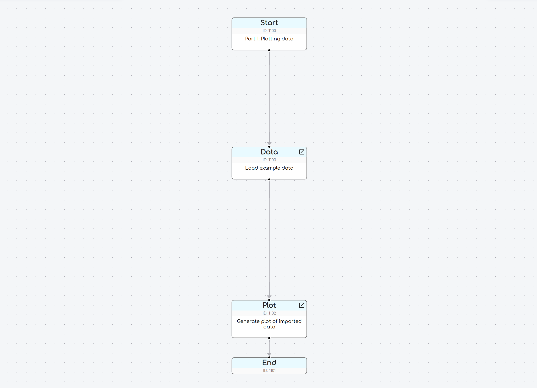
Create a new gridmo Project and add the following Nodes:
- Start Node
- Data Node
- Plot Node
- End Node
And connect the Nodes together as shown below.
1.3: Configure the Data Node
- Double click on the Data Node to open the configuration window.
- Set the
Input file namefield to the relative path of the .csv file you want to import, such asgridmo\data\e002_q_step1_data.csv. - Switch to the
Define outputstab. - Add the following OUTPUT commands to convert the columns in the .csv file to Internode Variables for use in gridmo.
// Convert from CSV column names into Internode Variables
OUTPUT, COL=V_pu, NAME=i_ch_poc_v
OUTPUT, COL=P_MW, NAME=i_ch_poc_p
OUTPUT, COL=Q_MVAr, NAME=i_ch_poc_q
The above commands convert each column from the name in the .csv file to an Internode Variable for use in gridmo. Specifically:
- The column
V_pucan be accessed by Nodes connected to this Data Node usingi_ch_poc_v. - The column
P_MWcan be accessed by Nodes connected to this Data Node usingi_ch_poc_p. - The column
Q_MVArcan be accessed by Nodes connected to this Data Node usingi_ch_poc_q.
If your .csv file is using a different unit than the unit you want for your simulation, you can use the optional argument VALSCALE= to apply a multiplicative scale.
You do not need to directly modify the source .csv file.
For example, if you .csv data file has voltage in kV (with a 33 kV base) you can use the following command:
OUTPUT, COL=V_at_33kV, NAME=i_ch_poc_v, VALSCALE=1/33
1.4: Configure the Plot Node
- Double click on the Plot Node to open the configuration window.
- Enter an output file name, such as
Overlaying Data\Part 1 - Plotting data. - Select
Document (.pdf)andInteractive visualisation (.html)to output PDF and HTML files. - Enter a plot title, such as
E002 - Overlaying results with real-world data. - Enter a plot subtitle, such as
Part 1: Plotting data. - In the
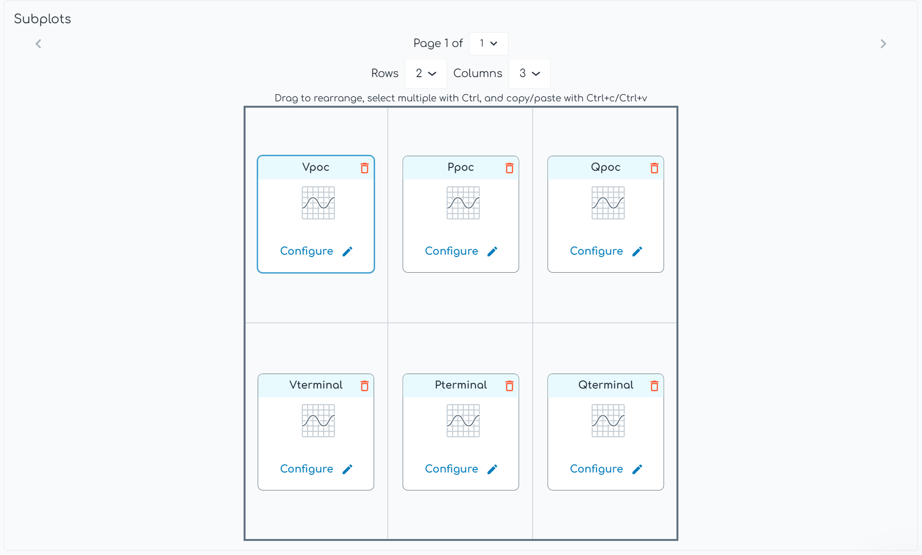
Define Subplotstab:- Set the
x-axis Minto 0 andx-axis Maxto 20. - Under
Subplotsselect 1 page, 2 rows and 2 columns. - Click on the
+to add a new subplot forVpoc,PpocandQpoc. For each subplot:- Enter a title in
Subplot title, such asVpoc. - Under
y-axis Channelsenter each of the Internode Variables with the double curly brackets, such as{{i_ch_poc_v}}
- Enter a title in
- Set the
1.5: Launch the simulation and review the results
- Launch the simulation.
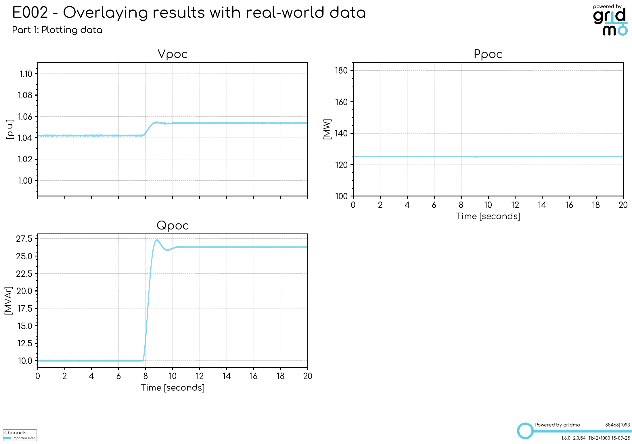
- The output plot should show the real-world data you imported plotted as per your configuration of the Plot Node.
- We can see in our outputs folder (example below) that we have plotted the real-world data:
- ✅ Point of connection voltage, active power and reactive power are all plotted.
- ✅ We can see in our data that the test being recorded appears to be a single reactive power step from 10 MVAr to about 26 MVAr.
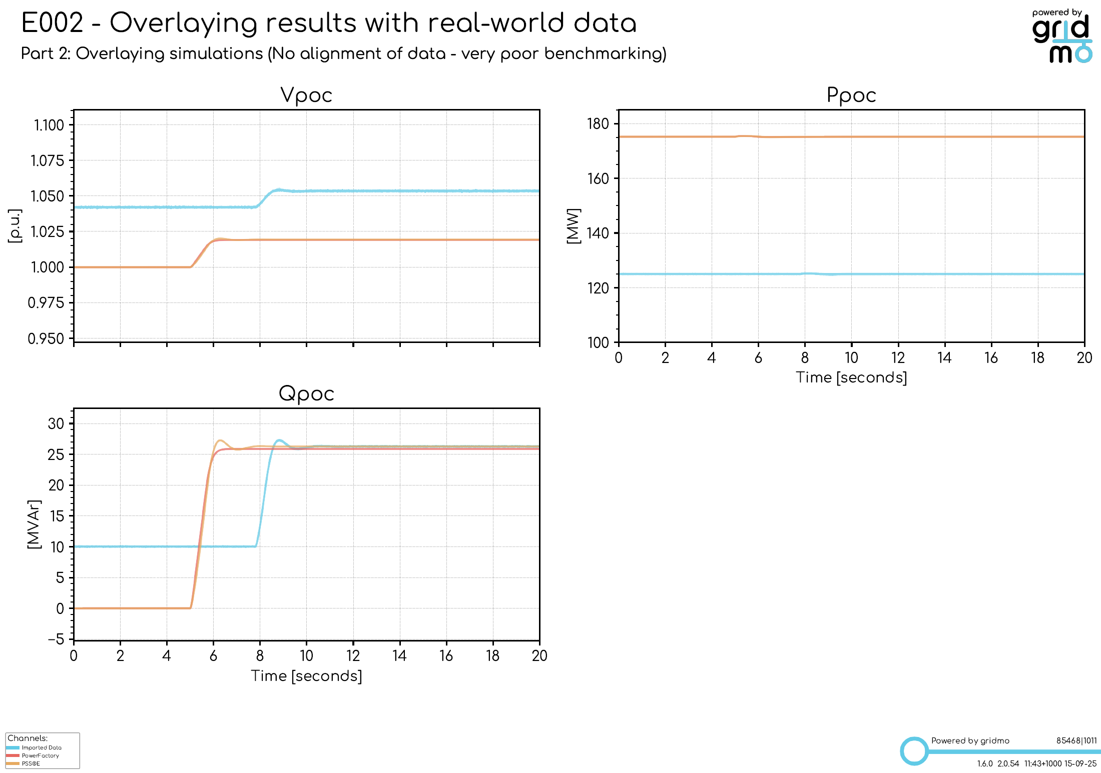
Part 2: Overlaying simulations
Now that we have imported real-world data, we will overlay this with the results of a dynamic study in PSS®E or PowerFactory. This is a common task when benchmarking dynamic simulations against real-world data.
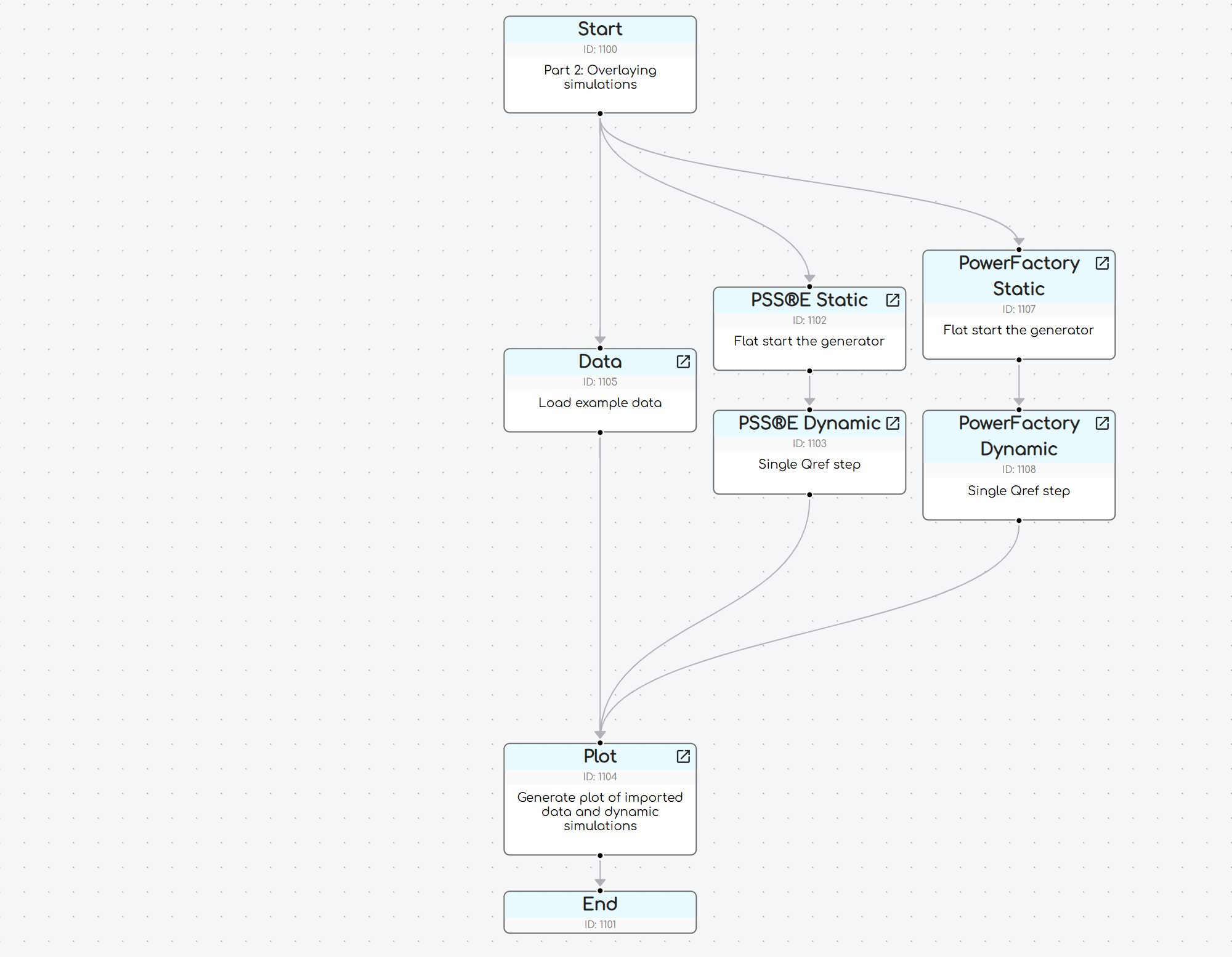
2.1: Add PSS®E / Powerfactory Nodes to your existing Run
- PSS®E Static Node (or PowerFactory Static Node).
- PSS®E Dynamic Node (or PowerFactory Dynamic Node).
2.2: Connect the Nodes
- The PSS®E Static Node should be connected to the PSS®E Dynamic Node (or PowerFactory Static Node to the PowerFactory Dynamic Node).
- The existing Data Node should be connected from the Start Node to the Plot Node.
- The PSS®E Dynamic Node (or PowerFactory Dynamic Node) should also be connected to the Plot Node.
2.3: Configure the PSS®E Static / PowerFactory Static Node
PSS®E
- In the
Select modeltab, set theModeltogridmo\wecc-solar\psse\solar.savto use an example 175 MW solar farm's PSS®E case file. - In the
Define simulation & Define outputstab, add the commands below to theCommandsfield, which describe what we want the PSS®E model to initialize to:
// Begin PSSE static simulation

// Set the Thevenin equivalent source impedance such that SCR is 7.5 and X/R is 4
SET, LINE=1000->999#1, STATUS=IN, SCR=7.5, XR=4

// Configure Vpoc as 1.0
// NOTE: The Thevenin equivalent voltage source (i.e. swing bus) is controlled to achieve the desired Vpoc target.
CONTROL, GEN=999#1, Q=VDIRECT, ATBUS=1000, QMIN=-9999, QMAX=9999, VTARGET=1.00

// Configure Ppoc and Qpoc of our solar farm such that Ppoc = 175 MW and Qpoc = 0 MVAr
CONTROL, GEN=91003#S1, ATLINE=1001->1000#1, P=175
CONTROL, GEN=91003#S1, ATLINE=1001->1000#1, Q=FIXED, QTARGET=0

// Solve the case
//NOTE: The SOLVE Command slowly resolves all CONTROL commands at the same time.
SOLVE
PowerFactory
- In the
Select modeltab, set theModeltogridmo\wecc-solar\dpf\wecc-solar.pfdto use an example 175 MW solar farm's PSS®E case file. - In the
Define simulation & Define outputstab, add the commands below to theCommandsfield, which describe what we want the PowerFactory model to initialize to:
// Begin PowerFactory static simulation

// Set the Thevenin equivalent source impedance such that SCR is 7.5 and X/R is 4
SET, LINE=POC->THEV#Zth, STATUS=IN, SCR=7.5, XR=4

// Configure Vpoc as 1.0
// NOTE: The Thevenin equivalent voltage source is controlled to achieve the desired Vpoc target.
SET, OBJECT_NAME=Load Flow Controller - Vpoc, VARIABLE=usetp, VAL=1.00

// Configure Ppoc and Qpoc of our solar farm such that Ppoc = 175 MW and Qpoc = 0 MVAr
SET, OBJECT_NAME=Power-Frequency Controller, VARIABLE=psetp, VAL=175
SET, OBJECT_NAME=Station Control, VARIABLE=qsetp, VALSCALE=-1, VAL=0

// Solve the case
SOLVE
The above commands:
- Set the SCR and X/R ratio for this example SMIB model to 7.5 and 4 respectively.
- Control the example solar farm to achieve P=175 MW, Q=0 MVAr at the solar farm's connection point.
- Use the infinite bus generator to achieve 1.00 pu voltage at the connection point.
2.4: Configure the PSS®E Dynamic / PowerFactory Dynamic Node
PSS®E
- Select the tickbox to enable
Use model from linked PSS®E Static Node. - Set the
Dynamics model datatogridmo\wecc-solar\psse\solar.dyrto use an example 175 MW solar farm's PSS®E dynamic data record. - In the
Define simulationtab:- Set the
Simulation time [seconds]to 20 seconds. - Add the following commands into the
Actionsfield:
- Set the
// Put solar farm in Q control mode
CONTROL, AT=0, ICON=M+5, GEN=91003#S1, DYRMODEL=REPCA1, VAL=0

// Complete a Qref step at 5 seconds
// NOTE: REPCA1 model definition, VAR (L+1) = Reactive power reference (Qref).
// NOTE: VALSCALE=1/200 for the Qref Command since values are specified on MBASE (200 MVA).
CONTROL, GEN=91003#S1, DYRMODEL=REPCA1, VAR=L+1, VALSCALE=1/200, AT=5, VAL=26.25
- In the
Define outputstab, add the following outputs:
OUTPUT, BUS=1000, VAL=V, NAME=i_ch_poc_v
OUTPUT, LINE=1001->1000#1, VAL=P, NAME=i_ch_poc_p
OUTPUT, LINE=1001->1000#1, VAL=Q, NAME=i_ch_poc_q
PowerFactory
- Select the tickbox to enable
Use model from linked PowerFactory Static Node. - Set the
Dynamics user modelstogridmo\wecc-solar\to use an example 175 MW solar farm's PowerFactory dynamic models. - In the
Define simulationtab:- Set the
Simulation time [seconds]to 20 seconds. - Add the following commands into the
Actionsfield:
- Set the
// Put solar farm in Q control mode
CONTROL, OBJECT_NAME=REPC_A Plant Control, VARIABLE=RefFlag, AT=-1, VAL=0

// Complete a Qref step at 5 seconds
// NOTE: REPC_A Plant Control model definition, Qrefp = Reactive power reference (Qref).
// NOTE: VALSCALE=1/200 for the Qref Command since values are specified on MBASE (200 MVA).
CONTROL, OBJECT_NAME=REPC_A Plant Control, VARIABLE=Qrefp, VALSCALE=1/200, AT=5, VAL=26.25
- In the
Define outputstab, add the following outputs:
OUTPUT, BUS=POC, VAL=V, NAME=i_ch_poc_v
OUTPUT, LINE=POC->THEV#Zth, VAL=P, NAME=i_ch_poc_p
OUTPUT, LINE=POC->THEV#Zth, VAL=Q, NAME=i_ch_poc_q
- The above commands:
- Set the solar farm's controller into fixed reactive power reference mode.
- Set the initial active power to 175 MW and sets the initial reactive power to 0 MVAr.
- Perform a single reactive power reference step at 5 seconds from 0 MVAr to 26.25 MVAr.
- Measure the voltage magnitude at the connection point and assign the name
i_ch_poc_v. - Measure the active power at the connection point and assign the name
i_ch_poc_p. - Measure the reactive power at the connection point and assign the name
i_ch_poc_q.
As we are naming the outputs i_ch_poc_v, i_ch_poc_p and i_ch_poc_q - which are the same as the names we defined as the outputs of the Data Node - we do not need to make any changes to the Plot Node.
The Plot Node will automatically plot all connected Nodes with the same output names on the same subplot, benchmarking the imported data, PSS®E Dynamic simulation and PowerFactory Dynamic simulation results.
2.5: Launch the simulation and review results
- Launch the simulation.
- We can see in our outputs folder (example below) that we have plotted the real-world data against the dynamic simulation results:
- ✅ There is a reactive power step in the PSS®E, PowerFactory and the real-world data
- ⚠️ The benchmarking is really poor. The reactive power steps are done at different times during the simulation and the initial active power isn't 175 MW, the initial reactive power isn't 0 MVAr and the POC voltage magnitude isn't 1.00 pu.
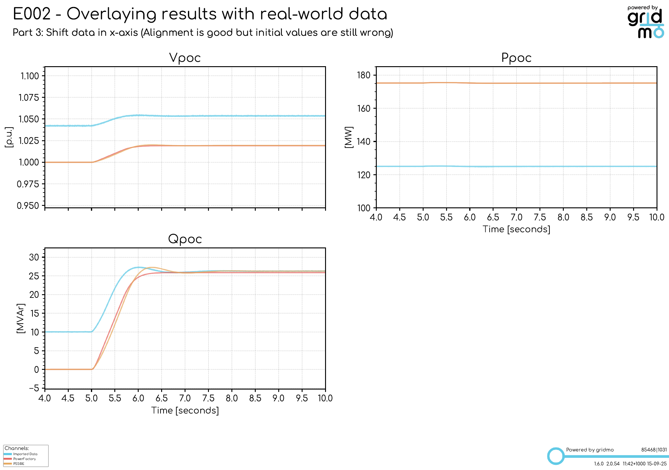
Part 3: Shift data in x-axis
In this part, we will use the Data Node's alignment capability to improve the benchmark with the PSS®E result.
In the previous section, we overlayed the dynamic simulation results with our real-world data and saw a very poor benchmark, as the time of the reactive power step in the data was different to the time in simulation. This is because it is very hard to have an event happen in real life at a specific time after starting to record data (e.g. exactly 5 seconds after starting meter recording). To improve this, we need to review our real-world data, find the index at which the event occurs and shift the data accordingly.
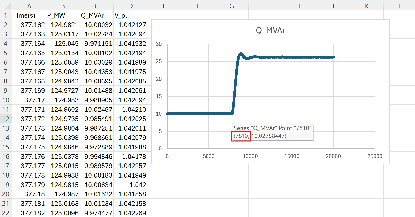
3.1: Open the source data in Excel to find the index of the step
You can find the example data in your gridmo Engine's Inputs folder in the gridmo folder at ...\gridmo\data\. The file we are using for this example is e002_q_step1_data.csv.
We can see:
- The time column starts from approximately 377 seconds, an arbitrary number. Having arbitrary date/time values is relatively common for real-world data which use a timestamp or similar (e.g. data doesn't always start at 0 seconds).
- By creating a 2-D line plot using the
Q_MVArcolumn, we can see that the reactive power step occurs at an index (row number in Excel) of approximately7810. - Our aim is to tell the gridmo platform to shift the real-world data so that the reactive power step occurs at a defined time in the 'simulation' world e.g. at same time as the PSS®E or PowerFactory simulation.
gridmo uses row indices (numbers) instead of time values for alignment.
This is because:
- The data might be in a complex timestamp format, which is common if exported from an Elspec PQM (for example
17/04/2024 7:15:32 PM). This adds unnecessary calculation burden to convert a timestamp into seconds since start of a simulation. - Even if the data is in a simple format like seconds (similar to our example data), requiring a time offset requires extra calculations on your behalf if the data doesn't start at 0 seconds. This is especially common if exported from real-world data.
3.2: Configure the Data Node to use manual alignment mode
- In your existing Run, double click on the Data Node.
- Select the
Process datatab in the Node configuration window. - Select
Manual alignbutton in theX-axis shiftarea.- In the
Row numberfield enter the row we found from excel, in our example7810. - In the
Time [seconds]field enter the time in seconds that the step occurs in the simulation, in our example5seconds.
- In the
- Click
Applyto save the changes.
We have now configured the Data Node to shift the real-world data so that the reactive power step occurs at 5 seconds in the simulation world.
3.3: Configure the PSS®E Dynamic / PowerFactory Dynamic Node and Plot Node to have a shorter simulation time
Now that we've shifted the real-world data, we can update the PSS®E Dynamic, PowerFactory Dynamic and Plot Nodes to have a shorter simulation time.
- Double click on the PSS®E Dynamic / PowerFactory Dynamic Node.
- Under the
Define simulationtab, set theSimulation time [seconds]to10seconds. - Click
Applyto save the changes. - Double click on the Plot Node.
- Under the
Define subplotstab, set thex-axis Min [seconds]to4and thex-axis Max [seconds]to10. - Click
Applyto save the changes.
3.4: Launch the simulation and review results
- Launch the simulation.
- We can see in our outputs folder (example below) that our real-world data has been shifted:
- ✅ The reactive power step now occurs at 5 seconds in the simulation.
- ⚠️ The benchmarking is better, but still poor (initial active power, reactive power and voltage are still incorrect) .
Part 4: Initialize simulations from data
In this part, we will initialize the dynamic simulations from the initial values of the imported data. We're going to modify our Flow so that we can export values from the Data Node into PSS®E Static / PowerFactory Static Node. This will allow us to use the initial values from the real-world data.
4.1: Modify your Run such that the PSS®E Static / PowerFactory Static Node is linked to the Data Node
Update your gridmo Run by dragging Nodes (left click and drag) and deleting edges (left click, then press the Delete key) so that the PSS®E Static / PowerFactory Static Node depends on the Data Node as shown below.
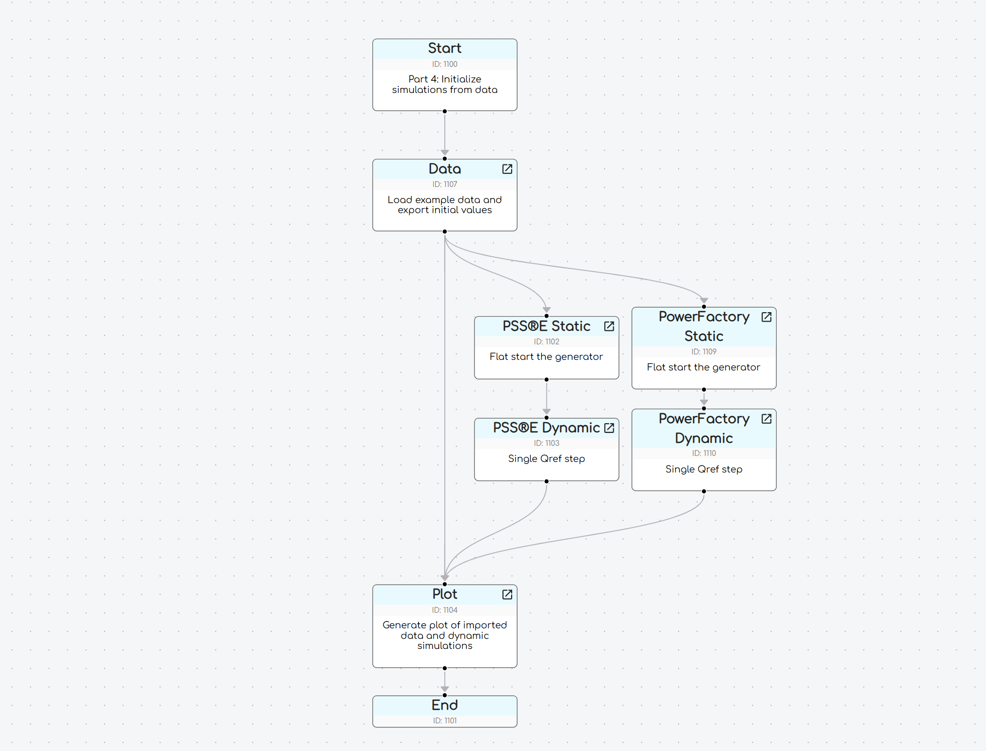
In our re-arranged Run, the Data Node is still connected to the Plot Node and we do not require any changes to the Plot Node for this step.
4.2: Configure the Data Node to export the initial values
- Double click on the Data Node.
- Select the
Define outputstab in the Node configuration window. - Add the following rows in addition to those which already exist in this field.
// Export values at the start of the data - note the AT=0 arguments have been added
OUTPUT, COL=V_pu, NAME=i_ch_poc_v_initial, AT=0
OUTPUT, COL=P_MW, NAME=i_ch_poc_p_initial, AT=0
OUTPUT, COL=Q_MVAr, NAME=i_ch_poc_q_initial, AT=0
- The above
OUTPUTcommands has the optionalAT=argument, which means export the single value instead of the entire column of data. We have set them to output at 0 seconds (after being shifted by the manual alignment mode we turned on in the previous step). Specifically:- The Internode Variable
i_ch_poc_v_initialstores the initial voltage from the Data Node (in per unit - the same unit as the in the .csv file). - The Internode Variable
i_ch_poc_p_initialstores the initial active power from the Data Node (in MW - the same unit as the in the .csv file). - The Internode Variable
i_ch_poc_q_initialstores the initial reactive power from the Data Node (in MVAr - the same unit as the in the .csv file).
- The Internode Variable
- Click
Applyto save the changes
4.3: Configure the PSS®E Static / PowerFactory Static Node to use the new Internode Variables
Now that the Data Node is exporting the initial values, we can update the PSS®E Static / PowerFactory Static Node to use these values.
PSS®E
- Double click on the PSS®E Static Node.
- Select the
Define simulation & Define outputstab in the Node configuration window. - Replace the commands in the
Commandsfield with the following (the lines which have changed from the previous steps are highlighted):
// Begin PSSE static simulation

// Set the Thevenin equivalent source impedance such that SCR is 7.5 and X/R is 4
SET, LINE=1000->999#1, STATUS=IN, SCR=7.5, XR=4

// Configure Vpoc, Ppoc and Qpoc using values imported from the Data Node
// NOTE: The Thevenin equivalent voltage source (i.e. swing bus) is controlled to achieve the desired Vpoc target.
CONTROL, GEN=999#1, Q=VDIRECT, ATBUS=1000, QMIN=-9999, QMAX=9999, VTARGET={{i_ch_poc_v_initial}}
CONTROL, GEN=91003#S1, ATLINE=1001->1000#1, P={{i_ch_poc_p_initial}}
CONTROL, GEN=91003#S1, ATLINE=1001->1000#1, Q=FIXED, QTARGET={{i_ch_poc_q_initial}}

// Solve the case
//NOTE: The SOLVE Command slowly resolves all CONTROL commands at the same time.
SOLVE
PowerFactory
- Double click on the PowerFactory Static Node.
- Select the
Define simulation & Define outputstab in the Node configuration window. - Replace the commands in the
Commandsfield with the following (the lines which have changed from the previous steps are highlighted):
// Begin PowerFactory static simulation

// Set the Thevenin equivalent source impedance such that SCR is 7.5 and X/R is 4
SET, LINE=POC->THEV#Zth, STATUS=IN, SCR=7.5, XR=4

// Configure Vpoc, Ppoc and Qpoc using values imported from the Data Node
// NOTE: The Thevenin equivalent voltage source is controlled to achieve the desired Vpoc target.
SET, OBJECT_NAME=Load Flow Controller - Vpoc, VARIABLE=usetp, VAL={{i_ch_poc_v_initial}}
SET, OBJECT_NAME=Power-Frequency Controller, VARIABLE=psetp, VAL={{i_ch_poc_p_initial}}
SET, OBJECT_NAME=Station Control, VARIABLE=qsetp, VALSCALE=-1, VAL={{i_ch_poc_q_initial}}

// Solve the case
SOLVE
- The above commands:
- Set the SCR and X/R ratio for this example SMIB model to 7.5 and 4 respectively.
- It then controls the example solar farm to achieve an active power and reactive power from the Internode Variables
i_ch_poc_p_initialandi_ch_poc_q_initialwe defined in the Data Node above. - It also uses the infinite bus generator to achieve a voltage at the connection point as per the
i_ch_poc_v_initialInternode Variable.
- Click
Applyto save the changes
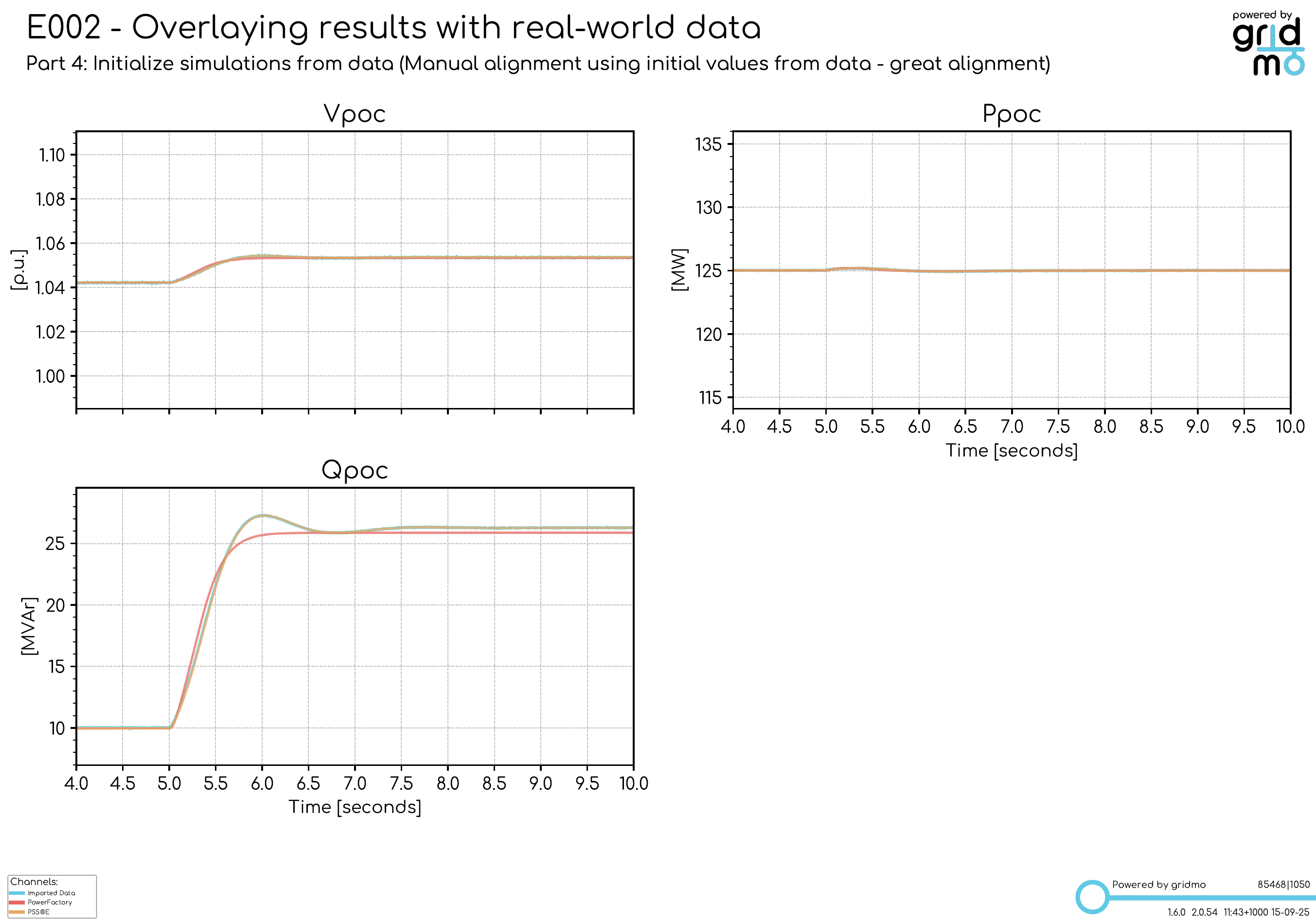
4.4: Launch the simulation and review results
- Launch the simulation.
- We can see in our outputs folder (example below) that our real-world data has been shifted:
- ✅ The reactive power step occurs at 5 seconds in the simulation.
- ✅ The initial values of the POC voltage, active power and reactive power now match between the real-world data and the dynamic simulation.
Part 5: Multiple tests with loops
In this part, we will use a Loop: Start Node to set up multiple tests. This is useful for creating overlays for different tests (such as different Qref steps), importing different data files or varying other test variables such as simulation length.
For this example, we will be adding an additional test to our existing Run, with a reactive power step down to -26.25 MVAr at 5 seconds, using a different data file.
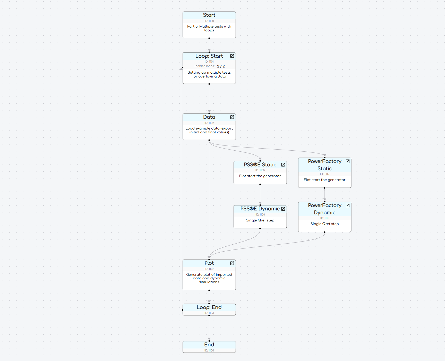
5.1: Add Loop: Start and Loop: End Nodes and modify your Run
Add the following Nodes to your project:
- Loop: Start Node
- Loop: End Node
Re-arrange your Run to wrap the existing Nodes within the Loop: Start and Loop: End Nodes and connect them as shown below:
5.2: Configure the Loop: Start Node
- Double click on the Loop: Start Node.
- Delete the 3rd row (which was added by default) so that there are two rows (Loops) and add new Loop Variables such that there are 8 Loop Variables in total.
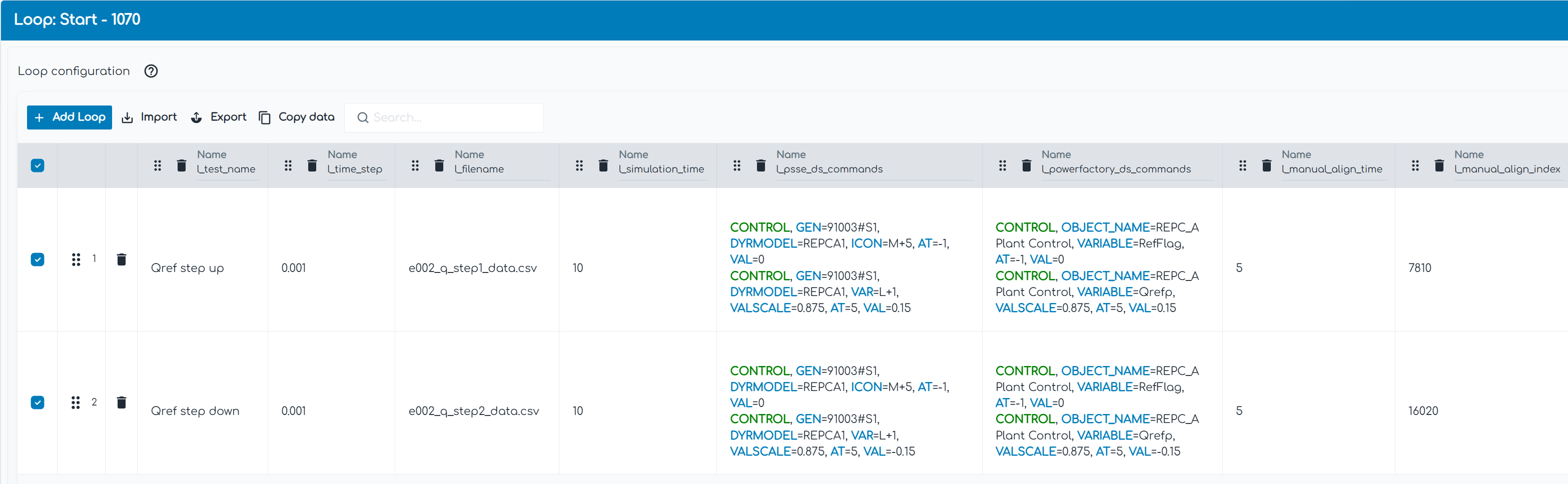
- Rename each Loop Variable (at the top of the column) as follows:
l_test_namel_time_stepl_filenamel_simulation_timel_psse_ds_commandsl_powerfactory_ds_commandsl_manual_align_timel_manual_align_index
- Fill in the fields of each Loop Variables with the following:
l_test_name: EnterQref step upfor Loop 1 andQref step downfor Loop 2.l_time_step: Enter0.001for both Loops.l_filename: Entere002_q_step1_data.csvfor Loop 1 ande002_q_step2_data.csvfor Loop 2.l_simulation_time: Enter15for both Loop 1 and Loop 2.l_manual_align_time: Enter5for both Loops.l_manual_align_index: Enter7810for Loop 1 and16020for Loop 2.
- For
l_psse_ds_commandsandl_powerfactory_ds_commands, enter the following commands for Loop 1:
CONTROL, GEN=91003#S1, DYRMODEL=REPCA1, ICON=M+5, AT=-1, VAL=0
CONTROL, GEN=91003#S1, DYRMODEL=REPCA1, VAR=L+1, VALSCALE=0.875, AT=5, VAL=0.15
CONTROL, OBJECT_NAME=REPC_A Plant Control, VARIABLE=RefFlag, AT=-1, VAL=0
CONTROL, OBJECT_NAME=REPC_A Plant Control, VARIABLE=Qrefp, VALSCALE=0.875, AT=5, VAL=0.15
- For Loop 2, enter the following for the
l_psse_ds_commandsandl_powerfactory_ds_commandsfields:
CONTROL, GEN=91003#S1, DYRMODEL=REPCA1, ICON=M+5, AT=-1, VAL=0
CONTROL, GEN=91003#S1, DYRMODEL=REPCA1, VAR=L+1, VALSCALE=0.875, AT=5, VAL=-0.15
CONTROL, OBJECT_NAME=REPC_A Plant Control, VARIABLE=RefFlag, AT=-1, VAL=0
CONTROL, OBJECT_NAME=REPC_A Plant Control, VARIABLE=Qrefp, VALSCALE=0.875, AT=5, VAL=-0.15
Your Loop: Start Node should now be configured as follows:
5.3: Configure the existing Nodes to use Loop Variables
We will now use these new Loop Variables within the existing Nodes in our Run.
Data Node
- Double click on the Data Node.
- In the
Input file namefield, replacegridmo\data\e002_q_step1_data.csvwithgridmo\data\$l_file_name. - Switch to the
Process datatab. - In the
Row numberfield, replace7810with$l_manual_align_index. - In the
Time [seconds]field, replace5with$l_manual_align_time.
PSS®E Dynamic / PowerFactory Dynamic Node
- Double click on the PSS®E Dynamic / PowerFactory Dynamic Node.
- For PSS®E Dynamic Node:
- Switch to the
Define simulationtab. - In the
Simulation time [seconds]field, enter the Loop Variable$l_simulation_time. - In the
Actionsfield, replace the existingCONTROLcommands with$l_psse_ds_commands.
- Switch to the
- For PowerFactory Dynamic Node:
- Switch to the
Define simulationtab. - In the
Simulation time [seconds]field, enter the Loop Variable$l_simulation_time. - In the
Actionsfield, replace the existingCONTROLcommands with$l_powerfactory_ds_commands.
- Switch to the
Plot Node
- Double click on the Plot Node.
- Switch to the
Define subplotstab and replace thex-axis: Maxfield with$l_simulation_time.
5.4: Launch simulation and review results
- Launch the simulation.
- We can see in our outputs folder that we have two plots for the two scenarios in our Loops.
- ✅ Loop 1 shows the reactive power step up at 5 seconds to approximately 26 MVAr.
- ✅ Loop 2 shows the reactive power step down at 5 seconds to approximately -26 MVAr.
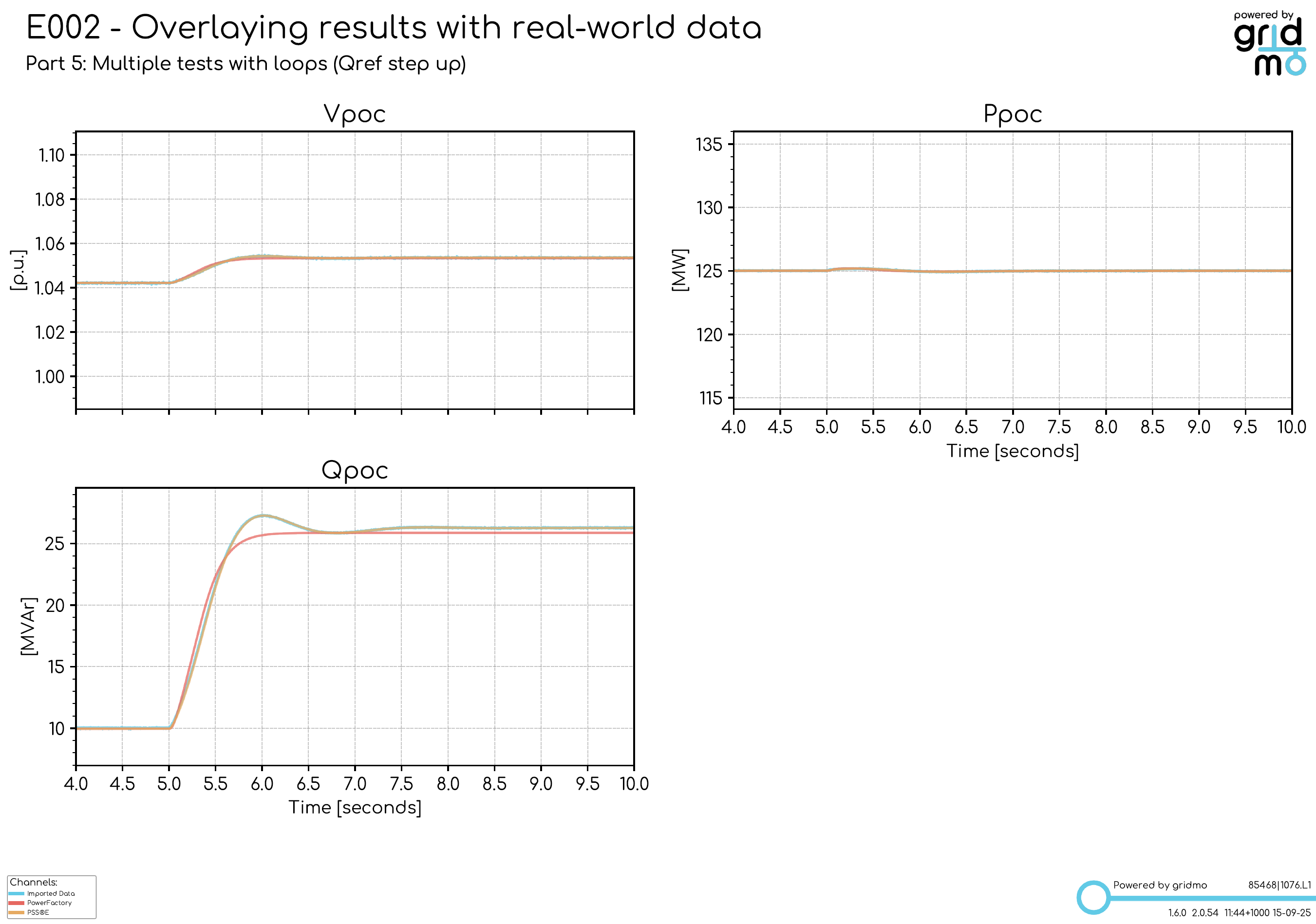
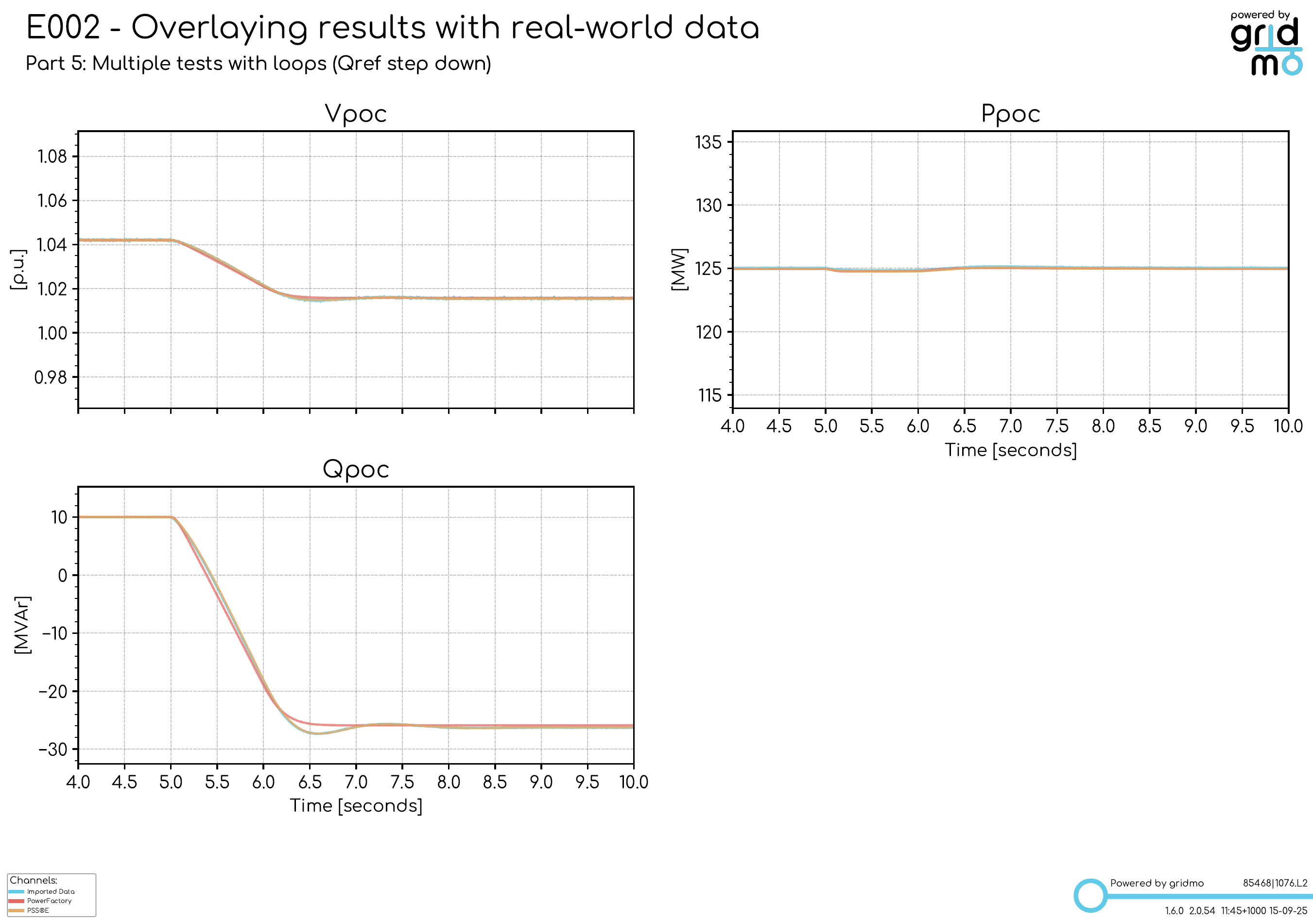
By using the Loop: Start Node, you can now setup multiple overlays in one place by modifying the Loop Variables for input data files, type of tests, simulation times, manual alignment indexes and the associated PSS®E and PowerFactory commands.
Part 6: Overlay builder
In this final part, we will add Overlay builder which makes it easy to configure the Loop: Start and Data Nodes in the previous example.
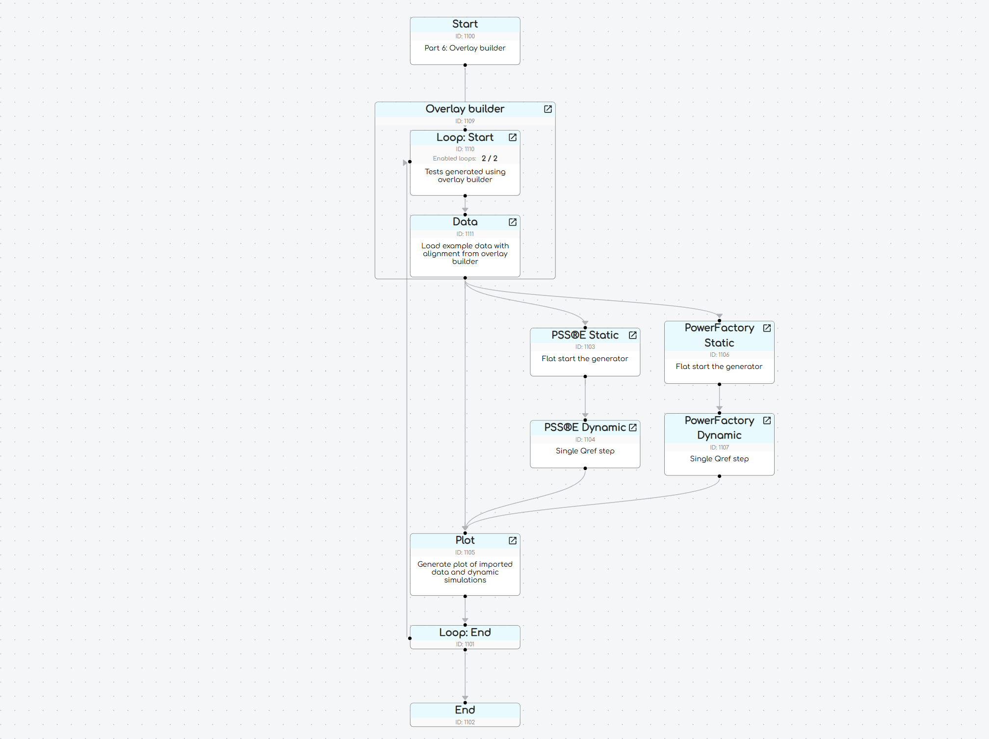
6.1: Add Overlay builder and modify Run
- Delete the Loop: Start and Data Nodes in your existing Run.
- Click on the '+' icon on the left-hand side and select Overlay builder under
Node Builders, and connect it between the Start Node and PSS®E Dynamic / PowerFactory Dynamic Nodes as follows:
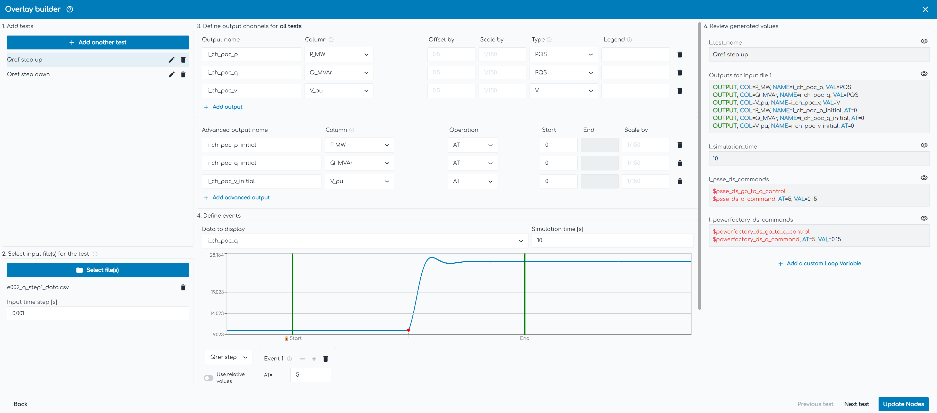
6.2: Configure Overlay builder
Setup
- Double click on the Overlay builder to open the Overlay builder window.
- Tick
PSS®EandPowerFactorycheckboxes underOverlay data with the following software. - Set the
Input folderfield togridmo\datadirectory which contains the example 175 MW solar farm's data, and clickNext.
Add tests and input data
- In the top-left corner, click
+ Add another testand rename the test using the pencil icon toQref step up. - Below
Add tests, click theSelect file(s)button and navigate to thegridmo\datadirectory and select thee002_q_step1_data.csvdata file. - In the
Input time step [s]field, enter0.001. TheDefine output channels for all testssection should now appear.
Define outputs
- In
Define output channels for all tests, clickAdd outputand then the dropdown underColumn. You should see here the column headings from the example .csv data file. SelectP_MW. - Now in the
Output namefield, enteri_ch_poc_pwhich is the Internode Variable name for active power. - In the
Typefield dropdown, selectPQS. - Repeat the above for:
Q_MVArwith output namei_ch_poc_qand selectPQSfor theType.V_puwith output namei_ch_poc_vand selectVfor theType.
- We will now extract the initial values of the data for initialising our dynamic simulations. Click
Add advanced outputand selectP_MWagain. - In the Start field, enter 0 (which means we will extract the active power value at T=0 seconds).
- In the
Advanced output namefield, enteri_ch_poc_p_initialwhich is the Internode Variable for the initial value of active power. - Repeat the above for:
Q_MVArwith output namei_ch_poc_q_initial.V_puwith output namei_ch_poc_v_initial.
Define events
We will now tell Overlay builder when the Qref step occurs and what commands to use for the dynamic simulations.
- In
Define events, click the dropdown underData to displayand selecti_ch_poc_qorQ_MVArand set theSimulation time [s]field to10. You will now see the reactive power data in graph. - To tell Overlay builder when the Qref step occurs, you can do the following:
- Click on the point at which the Qref step occurs directly, by selecting a point on the graph.
- Alternatively, click
Auto-generate eventswhich will automatically find the time at which Qref step occurs.
- Note that you can also adjust the point using the
- +buttons below the plot in theEvent 1box.
Now that we have recorded the time at which the Qref step occurs, we need to tell Overlay builder the final value of Q_MVAr. From the graph, we can see this value is around 26.25 MVAr. However, our model receives the reactive power reference command in per unit on a base of 175 MW (the plant's rated capacity). Hence, our Qref command will be 26.25/175 = 0.15 pu.
- In the
Event 1box in theVAL=field, enter0.15.
We will now configure the second test which has a reactive power reference step down to -26.25 MVAr.
- Add the second test by clicking
+ Add another testand name itQref step down. - Click
Select file(s)and add the same .csv data file as the first testgridmo\data\e002_q_step2_data.csv. - Set the
Input time step [s]field to 0.001. - Note that all the output channels configured for the first test are already pre-populated for the second test.
- In
Define events, selecti_ch_poc_qunderData to displayand repeat the same steps as the first test but this time defining an event withAT=5andVAL=-0.15.
Review generated values
In the Review generated values section on the right-hand side, you will now see the generated Loop Variables used for the dynamic simulation.
Overlay builder will automatically generate commands to configure the PSS®E command Loop Variable l_psse_ds_commands and PowerFactory command Loop Variable l_powerfactory_ds_commands using your project's Global Variables.
Your Overlay builder window should now look as below:
Generate Nodes
- Finish the Overlay builder setup by clicking
Generate Nodeson the bottom-right corner. - You will now be able to view the configured Loop: Start and Data Nodes within the Overlay builder box. Notice here that these Nodes are identical to the Loop: Start and Data Nodes from Step 5, which we set up manually without Overlay builder.
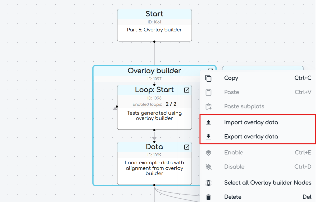
If you open an Overlay builder Node and you are unable to find your input data, you will need to select the input files again as the Overlay builder does not save the input data files within the gridmo project file.
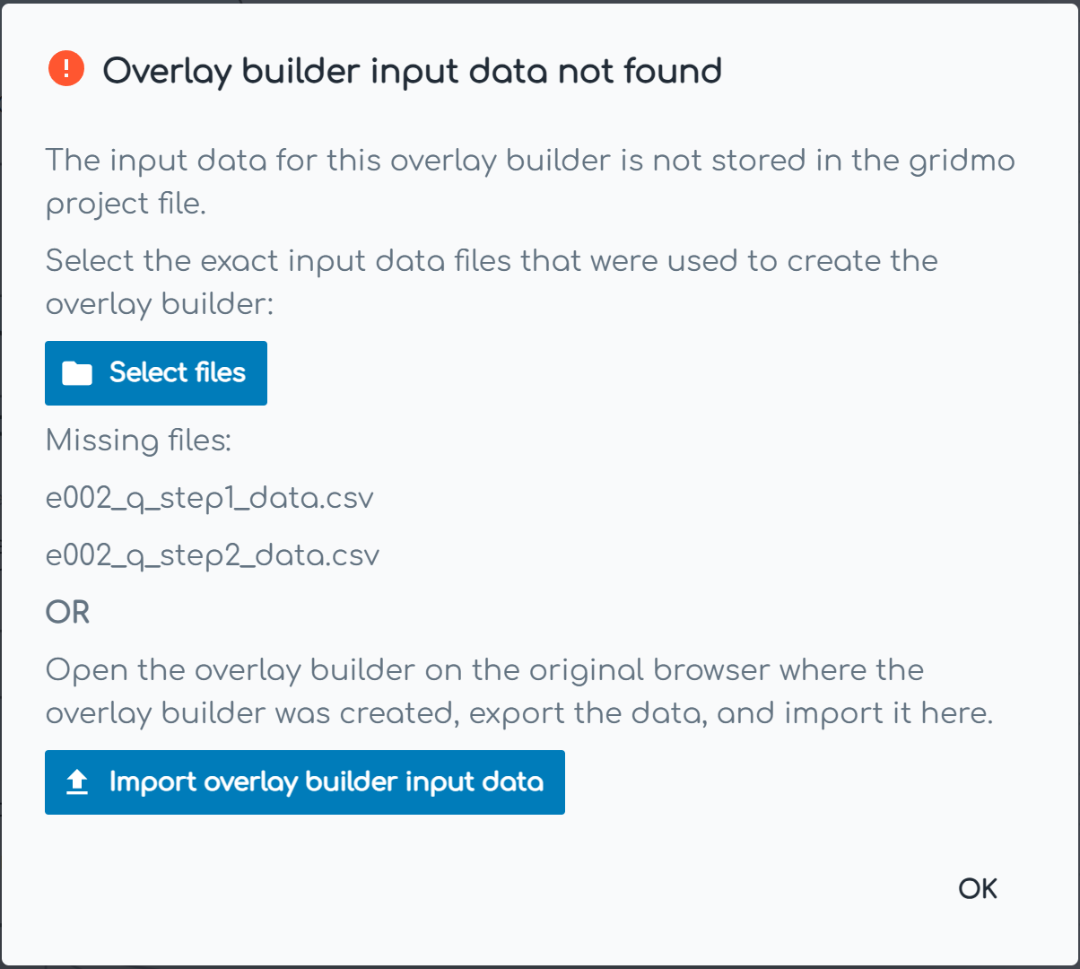
Alternatively, you can export the data files from the original browser where Overlay builder was created by right clicking on the Overlay builder Node and selecting Export overlay data. This will download a .json file which you can import into your current project by right clicking and selecting Import overlay data.
6.3: Launch simulation and review results
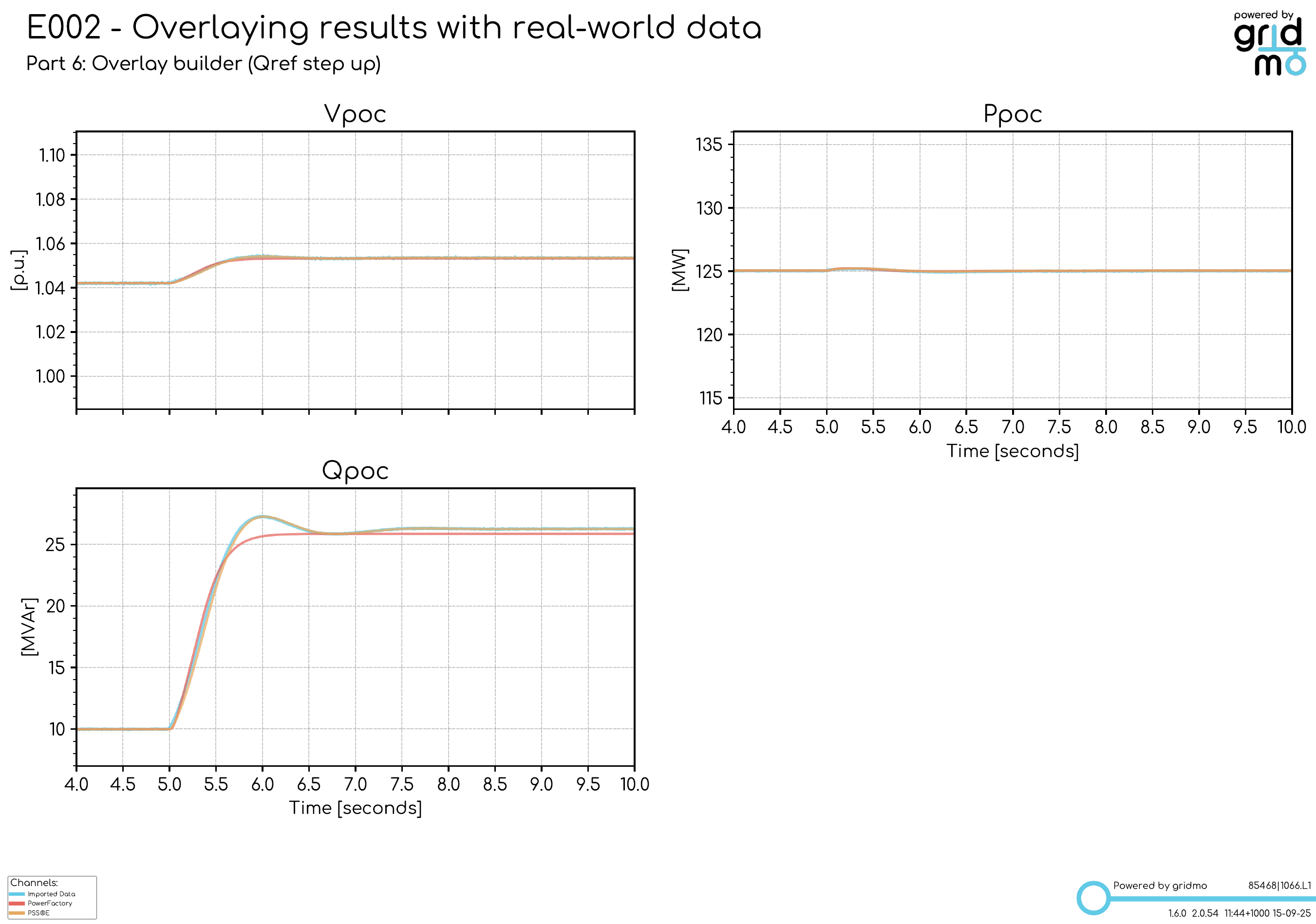
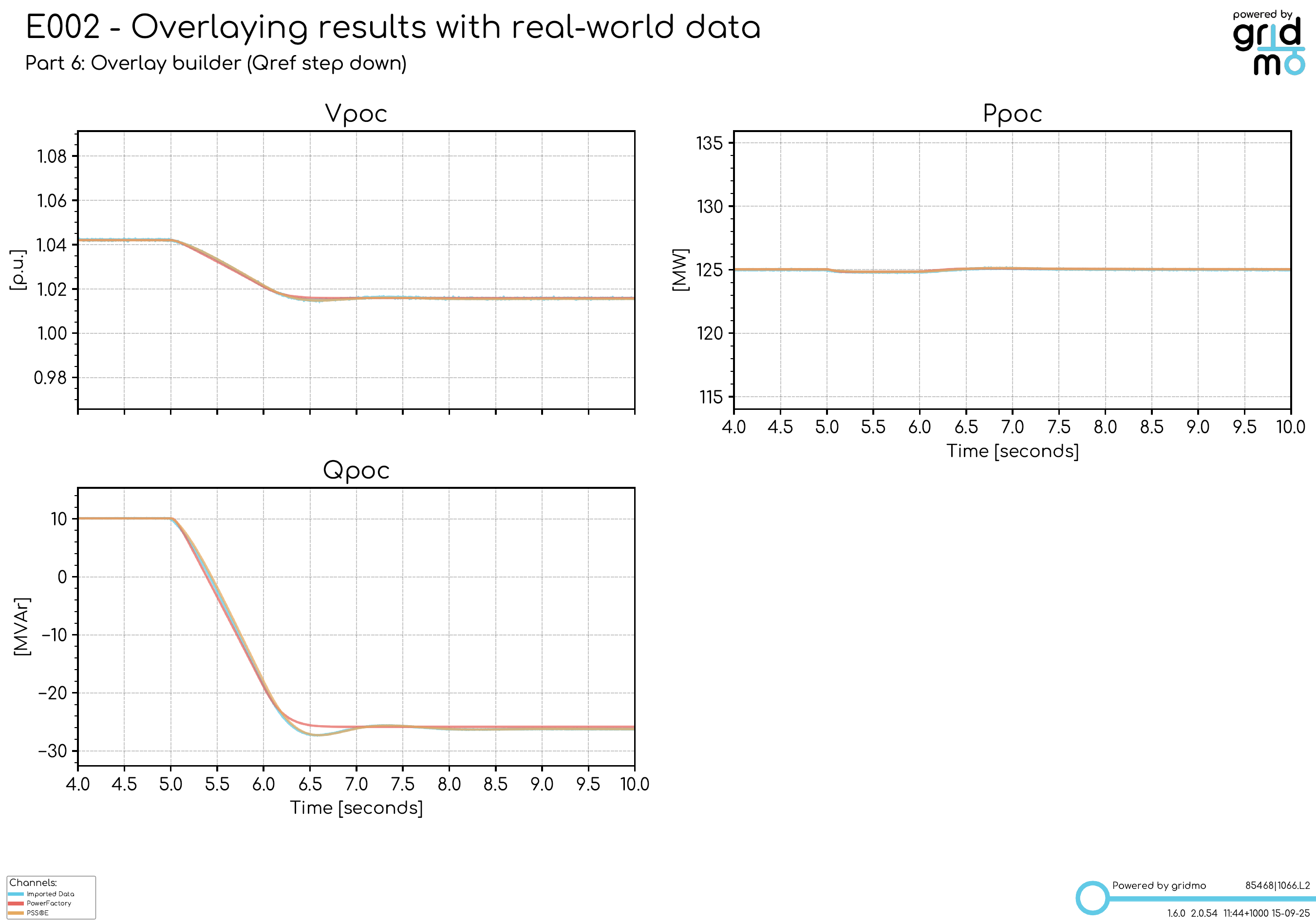
- Launch the simulation.
- We can see in our outputs folder that our plots are identical to Step 4, this time configured with Overlay builder.
- ✅ Loop 1 shows the reactive power step up at 5 seconds to approximately 26 MVAr.
- ✅ Loop 2 shows the reactive power step down at 5 seconds to approximately -26 MVAr.
Revision history
Version 3 | 21 September 2025
New- Added new Runs for importing from data (Part 1), initializing from data while using manual alignment (Part 4), multiple tests using loops (Part 5) and using Overlay builder (Part 6).
- Renamed 'No alignment' Run to 'Part 2: Overlaying simulations' and Manual alignment Run to 'Part 3: Shift data in x-axis', along with other updates required to use new data files.
- Removed outdated PowerFactory only and PSCAD™ only Runs, as well as PSS®E only Runs which used auto alignment.
Version 2 (v1.4.15.6) | 23 July 2024
- Updated Sticky Node helper text in example.
Version 1 (v1.4.15) | 20 June 2024
- First release of example file.