Plot
Introduction
The Plot Node analyzes data from connected Nodes and outputs results to other connected Nodes or outputs plots in a graphical format.
This Node is typically used for the following:
- Outputting dynamic study results (e.g. plotting the time-series response of voltage at a bus).
- Benchmarking two or more power system models against each other.
- Analyzing data (e.g. calculating settling time on a generator's reactive power output).
- Outputting scatter plots summarizing analyzed data (e.g. plotting a droop curve based on results from multiple dynamic studies).
User inputs
Define plot
Output file name
Defines the output directory and file name of the plot, excluding the file extension.
Example:
DMAT_Table_1
Each Plot Node represents a single output file. Output file names within a simulation must be unique.
As a result, Loop Variables and Internode Variables are not supported in the Output file name field.
Output file types
Defines the output file types. Currently, the Plot Node supports:
- [Optional] Portable Document Format (PDF)
- [Optional] Interactive Visualization (HTML)
- [Optional] Image (PNG)
Plot title
Defines the title of the plot.
Example:
Sunny Solar Farm
Plot subtitle
Defines the subtitle of the plot.
Example:
S5.2.5.4 - Frequency ramp to 52 Hz, 4 Hz/sec, minimum system strength
Define subplots
Type
Defines the type of plot to generate. Options:
Time series: Plot one or more sub-plots with a common horizontal (x) axis with time as the independent variable. All sub-plots share a common x-axis range. This is typically used for displaying time series data from dynamic studies.Scatter plot: Generic scatter plot of channels on an x-axis and y-axis. This is typically used for post-processing and analysis of simulation data.
x-axis: Channels
Defines the channel to be used as input data for the plot's x-axis. Channels are defined using Internode Variables from a connected Node. Multiple channels are supported and are entered on subsequent lines.
Example: Display the Q(V) droop curve generated by a connected Table Node (with data from a connected PSS®E Dynamic Node) with the following Data: voltage={{i_vpoc}} and reactive_power={{i_qpoc}}:
{{voltage}}
Internode Variable names do not need to be unique within a Run. If a Plot Node channel is defined as {{voltage}} and a Table Node has data from two connected Nodes (e.g. PSS®E Dynamic Node and a PSCAD™ Node) output Internode Variables with the same name of voltage, the Plot Node will plot both channels on the same scatter plot.
x-axis: Label
Defines the horizontal axis label of the plot.
Example:
V [p.u.]
x-axis: Scaling
Defines the scaling of the horizontal axis. Options:
Auto: Automatically scales the axis with reasonable whitespace for simplified analysis.Auto: Tight: Automatically scales the axis as far as possible.Manual: Fixed user-defined minimum and maximum values.
x-axis: Min
Defines the minimum displayed value on the horizontal axis. Only appears if x-axis: Scaling is set as Manual.
Example: Set the minimum value for the horizontal axis to 0.
0
🔢 Supports mathematical operations.
x-axis: Max
Defines the maximum displayed value on the horizontal axis. Only appears if x-axis: Scaling is set as Manual.
Example: Set the maximum value for the horizontal axis to 100.
100
🔢 Supports mathematical operations.
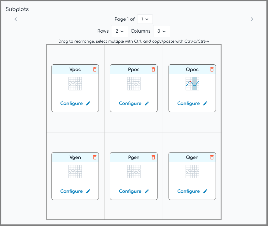
Subplot configuration space
Each plot may contain up to a maximum of 3 pages, each with 16 subplots. The grid displayed represents the layout of the subplots on a single page. Use the pages, rows and columns dropdowns to change this layout as desired. Click on the '+' icon to add a subplot, and click on the 'Configure' button to configure the subplot. Subplots can also be dragged to their preferred location on the page.
Subplot
Defines the subplot selection. Options:
Custom: Define a subplot which is custom to this particular Plot Node subplot.- Global subplot: Choose from an available global subplot.
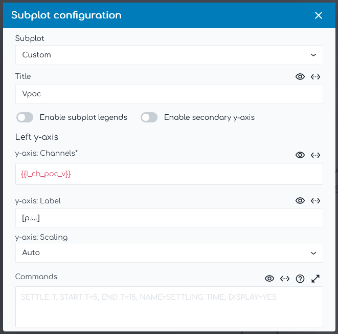
Title
Defines the title of the subplot.
Example:
Vpoc
Enable subplot legends
Enable or disable the display of legends on the subplot. Legend names are defined using the LEGEND Argument in OUTPUT Commands (e.g. PSS®E Dynamic Node - OUTPUT Command). Options:
Checked: Legend will appear on the subplot.Not checked: Legend will not appear on the subplot.
Enable secondary y-axis
Enable or disable the secondary y-axis on the subplot.
Checked: Subplot will allow a secondary y-axis.Not checked: Subplot will not allow a secondary y-axis.
Enable straight lines with scatter plot (Scatter Plot only)
Enable or disable straight lines connecting the scatter plot data. Options:
Checked: Scatter plot will include straight lines.Not checked: Scatter plot will not include straight lines.
You can configure channels on the left and right y-axes separately. Commands are only currently supported on left y-axis channels.
y-axis: Channels
Defines the channels which are used as input data for the subplot. Channels are defined using Internode Variables from a connected Node. Multiple channels are supported and are entered on subsequent lines.
Example: Display the time series data generated by a connected PSS®E Dynamic Node with the following Commands in its output field: OUTPUT, LINE=100->200#1, VAL=P, NAME=i_terminal_p and OUTPUT, LINE=400->500#1, VAL=P, NAME=i_poc_p.
{{i_terminal_p}}
{{i_poc_p}}
Internode Variable names do not need to be unique within a Run. If a Plot Node channel is defined as {{i_poc_p}} and two connected Nodes (e.g. PSS®E Dynamic Node and a PSCAD™ Node) output Internode Variables with the same name of P_POC, the Plot Node will plot both channels on the same subplot.
y-axis: Label
Defines the vertical axis label of the subplot.
Example:
V POC
y-axis: Scaling
Defines the vertical axis scaling of the subplot. Options:
Auto: Automatically scales the vertical axis based on the channel type with reasonable whitespace for simplified analysis.Auto: Tight: Automatically scale the vertical axis as far as possible.Manual: Fixed user-defined minimum and maximum values.
y-axis: Min
Defines the minimum displayed value on the vertical axis of the subplot. Only appears if y-axis: Scaling is set as Manual.
Example: Set the minimum value for the sub-plot vertical axis to 20.
20
🔢 Supports mathematical operations.
y-axis: Max
Defines the maximum displayed value on the vertical axis of the subplot. Only appears if y-axis: Scaling is set as Manual.
Example: Set the maximum value for the sub-plot vertical axis to 30.
30
🔢 Supports mathematical operations.
Commands
Defines the Commands which are applied to the subplot.
Supported Commands (Time Series):
- SETTLING_TIME: Calculates and optionally displays the settling time.
- RISE_TIME: Calculates and optionally displays the rise time.
- RECOVERY_T: Calculates and optionally displays the post-disturbance recovery time.
- EDGE: Outputs the time at which the channel rises to its maximum value or falls to its minimum value.
- COUNT_EDGES: Outputs the number of times a single channel in the subplot toggles between a low value and a high value.
- OUTPUT: Outputs a single value from each channel on the subplot at a specified time.
- ADVOUTPUT: Outputs data from each channel on the subplot with advanced features.
- ERROR_BAND: Calculates and displays an error band on the subplot using one channel as a reference.
- DRAW_LINE: Draws a line on the subplot with optional styling and shading.
- OSCILLATION_CALC: Calculates data about an oscillation such as frequency, damping ratio and damping factor.
Supported Commands (Scatter Plot):
- STYLE: Applies special styling to a scatter plot.
- GRADIENT: Calculates gradient of data on a scatter plot.
- DRAW_LINE: Draws a line on the subplot with optional styling and shading.
Advanced
Advanced Parameters
Advanced Parameters allow users to configure test details which are not commonly used. Advanced Parameters are often specific to each Node type.
Each line represents a new Advanced Parameter and is entered as a=b format, where a is the name of the Parameter and b is the corresponding value. All Advanced Parameters are set to their default values if they are not included in the Advanced Parameters field.
Example: Set Advanced Parameter, sample.parameter to a value of 5.
sample.parameter=5
API Reference
This section details the Commands and Advanced Parameters specific to the Node.
Commands
SETTLING_TIME | Calculate settling time
Also known as 'End of disturbance'.
SETTLING_TIME, START_T=, [END_T=], INITIAL_VAL=, FINAL_THRESHOLD_OVER=, FINAL_THRESHOLD_UNDER=, FINAL_VAL=, [FINAL_THRESHOLD_MIN=, FINAL_THRESHOLD_MIN=, HBANDS=NO, DISPLAY=YES, NAME=]
Calculates and optionally displays the settling time for each channel on the subplot. The calculation is the time taken for a signal to remain within a specified threshold of a final value. Threshold calculation methodology must be specified using available arguments and can differ between grid codes.
Arguments:
- SETTLING_TIME
- START_T 🔢 (
float): Start settling time calculation from this time [seconds]. - END_T (
float)[Optional]: End of the settling time calculation window [seconds]. The channel is expected to have reached its final value at this time (e.g. the end of the simulation or just prior to a further disturbance/controlled change). Defaults to the end of the channel data. Options:END_T=x🔢 wherexis afloat: End time isx.END_T=SIM_END: End time is the end of the simulation.
- INITIAL_VAL: Initial channel value used in threshold calculations. Options:
INITIAL_VAL=x🔢 wherexis afloat: Initial value isx.INITIAL_VAL=START_VAL: Initial value is the channel value atSTART_T.
- FINAL_THRESHOLD_OVER (
float %): The threshold around the final value (in the direction of the signal) where the signal is considered settled. When specified as a percentage, the value at which the settling time calculation finishes is the combination of two bands, the band specified by this argument is(final value) + (FINAL_VAL - INITIAL_VAL)*FINAL_THRESHOLD%. - FINAL_THRESHOLD_UNDER (
float %): The threshold around the final value (opposite to the direction of the signal) where the signal is considered settled. When specified as a percentage, the value at which the settling time calculation finishes is the combination of two bands, the band specified by this argument is(final value) - (FINAL_VAL - INITIAL_VAL)*FINAL_THRESHOLD%. - FINAL_VAL: Final channel value used in threshold calculations. Options:
FINAL_VAL=x🔢 wherexis afloat: Final value isx.FINAL_VAL=END_VAL: Final value is the channel value atEND_T.FINAL_VAL=MAX_ABS_OR_END_VAL: Automatically selects the value used in the threshold calculations based on the following criteria: If the sustained change (END_VAL - START_VAL) is less than half of the maximum change (MAX_ABS - START_VAL), the final value is MAX_ABS. Otherwise, the final value is END_VAL.
- FINAL_THRESHOLD_MIN 🔢 (
float) [Optional]: Minimum symmetrical threshold around the final value where the signal is considered settled. Often used in conjunction with INITIAL_VAL=START_VAL, FINAL_VAL=END_VAL and FINAL_THRESHOLD as a percentage because (FINAL_VAL - INITIAL_VAL)*FINAL_THRESHOLD% may become a very small number. - FINAL_THRESHOLD_MIN 🔢 (
float) [Optional]: Additional minimum symmetrical threshold. This argument may be repeated; each occurrence adds another minimum band constraint. See the first FINAL_THRESHOLD_MIN description above. - HBANDS (
bool)[Optional]: IfYES, adds four dotted horizontal lines corresponding to the values of INITIAL_VAL, FINAL_VAL and the two symmetrical final value thresholds. Defaults toNO(horizontal bands not shown). Only drawn ifDISPLAY=YES. - DISPLAY (
str)[Optional]: Display the settling time on the subplot and in the legend. Defaults toDISPLAY=YES. Options:DISPLAY=YES: Settling time will be displayed on the subplot and in the legend.DISPLAY=NO: Settling time will not be displayed on the subplot and in the legend.
- SHADE_COLOR (
str)[Optional]: Color of the shading of the subplot display. Defaults to a color complementary to the color of the line the calculation was completed on. Options:SHADE_COLOR=: CSS named color, reference the color using the 'Keyword' column here.SHADE_COLOR=RRGGBB: Hexadecimal color code.
- NAME (
str)[Optional]: Output the calculated settling time as an Internode Variable. Output names must be unique within a Node. - LEGEND (
str)[Optional]: Override the legend label to something other than "Settling time". E.g. "End of disturbance".
Example Diagram:
The diagram below shows an example SETTLING_TIME command.
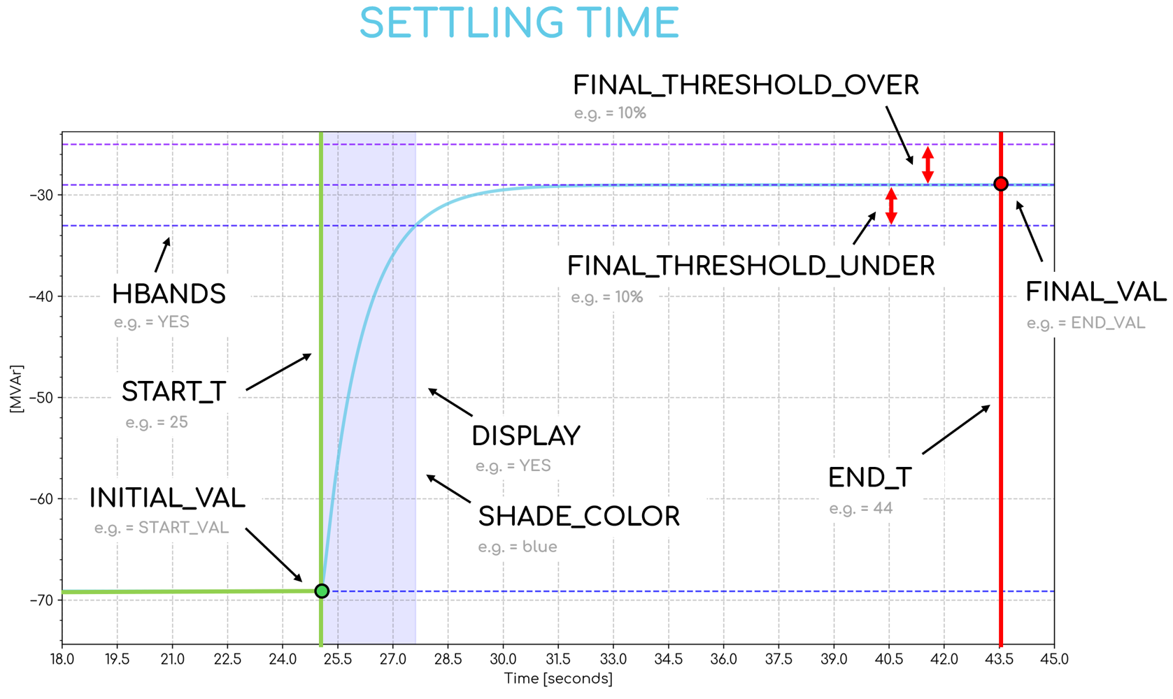
SETTLING_TIME, START_T=25, END_T=44, INITIAL_VAL=START_VAL, FINAL_THRESHOLD_OVER=10%, FINAL_THRESHOLD_UNDER=10%, FINAL_VAL=END_VAL, HBANDS=YES, DISPLAY=YES, SHADE_COLOR=blue
Example: Calculate the settling time for each channel on the subplot.
- Begin the calculation at 5 seconds, using the value at 5 seconds as the initial value.
- Automatically select the final value based on the following criteria:
- If the sustained change in the quantity is less than half of the maximum change in that output quantity, the maximum change induced in that output quantity; or
- The sustained change induced in that output quantity
- Calculate the time taken for the signal to settle from the initial value to within 10% of the final value
SETTLING_TIME, START_T=5, END_T=15, INITIAL_VAL=START_VAL, FINAL_THRESHOLD_OVER=10%, FINAL_THRESHOLD_UNDER=10%, FINAL_VAL=MAX_ABS_OR_END_VAL
Example: Calculate the settling time for each channel on the subplot.
- Begin the calculation at 5 seconds and assume the channels have reached a steady value by 15 seconds.
- Use the value at 5 seconds as the initial value.
- Use the value at 15 seconds as the final value.
- Calculate the time taken for the signal to settle from the initial value to within 10% of the final value, with a minimum band width of 3.2 MVAr.
SETTLING_TIME, START_T=5, END_T=15, INITIAL_VAL=START_VAL, FINAL_THRESHOLD_OVER=10%, FINAL_THRESHOLD_UNDER=10%, FINAL_VAL=END_VAL, FINAL_THRESHOLD_MIN=3.2
Example: Calculate the settling time for each channel on the subplot.
- Begin the calculation at 5 seconds and assume the channels have reached a steady value by 5.43 seconds.
- Use the value at 5 seconds as the initial value.
- Use the value at 5.43 seconds as the final value.
- Calculate the time taken from the initial value to when the signal stays within a band which is +20% and -10% of the final value, where the +20% band is the lower band assuming a falling signal.
SETTLING_TIME, START_T=5, END_T=5.43, INITIAL_VAL=START_VAL, FINAL_THRESHOLD_OVER=20%, FINAL_THRESHOLD_UNDER=10%, FINAL_VAL=END_VAL
RISE_TIME | Calculate rise time
Also known as 'Response time', 'Reaction time', 'Commencement time'.
RISE_TIME, START_T=, [END_T=], INITIAL_VAL=, INITIAL_THRESHOLD=, FINAL_THRESHOLD=, FINAL_VAL=, [END_MEAN_T=, HBANDS=NO, DISPLAY=YES, NAME=]
Calculates and optionally displays the rise time (or fall time) for each channel on the subplot. The calculation is the time taken for a signal to rise (or fall) from a specified threshold to a specified threshold. Threshold calculation methodology must be specified using available arguments and can differ between grid codes.
Arguments:
- RISE_TIME
- START_T 🔢 (
float): Start of the rise time calculation window [seconds]. - END_T[Optional]: End of the rise time calculation window [seconds]. The channel is expected to have reached its final value at this time (e.g. the end of the simulation or just prior to a further disturbance/controlled change). Defaults to the end of the channel data. Options:
END_T=x🔢 wherexis afloat: End time isx.END_T=SIM_END: End time is the end of the simulation.
- INITIAL_VAL: Initial channel value used in threshold calculations. Options:
INITIAL_VAL=x🔢 wherexis afloat: Initial value isx.INITIAL_VAL=START_VAL: Initial value is the channel value atSTART_T.
- INITIAL_THRESHOLD (
float %): The value at which the rise time calculation begins. When specified as a percentage, the value at which the rise time calculation begins is INITIAL_THRESHOLD% * (FINAL_VAL - INITIAL_VAL). - FINAL_THRESHOLD (
float %): The value at which the rise time calculation finishes. When specified as a percentage, the value at which the rise time calculation finishes is FINAL_THRESHOLD% * (FINAL_VAL - INITIAL_VAL). - FINAL_VAL: Final channel value used in threshold calculations. Options:
FINAL_VAL=x🔢 wherexis afloat: Final value isx.FINAL_VAL=END_VAL: Final value is the channel value atEND_T.FINAL_VAL=END_MEAN: Final value is the average of the values from (END_T-END_MEAN_T) to (END_T).FINAL_VAL=MAX: Final value is the maximum of the signal in the direction of the signal change (i.e. falling or rising).FINAL_VAL=MAX_ABS: Final value is the maximum absolute change of the signal irrespective of direction. This is sometimes referred to as "maximum change induced".
- END_MEAN_T (
float %)[Optional]: Used ifFINAL_VAL=END_MEAN. The time prior toEND_Tused in the average calculation. When specified as a percentage, the time is END_MEAN_T% * (END_T - START_T). - HBANDS (
bool)[Optional]: IfYES, adds four dotted horizontal lines corresponding to the values of INITIAL_VAL, INITIAL_THRESHOLD, FINAL_THRESHOLD, FINAL_VAL. Defaults toNO(horizontal bands not shown). Only drawn ifDISPLAY=YES. - DISPLAY (
str)[Optional]: Display the rise time on the subplot and in the legend. Defaults toDISPLAY=YES. Options:DISPLAY=YES: Rise time will be displayed on the subplot and in the legend.DISPLAY=NO: Rise time will not be displayed on the subplot and in the legend.
- SHADE_COLOR (
str)[Optional]: Color of the shading of the subplot display. Defaults to a color complementary to the color of the line the calculation was completed on. Options:SHADE_COLOR=: CSS named color, reference the color using the 'Keyword' column here.SHADE_COLOR=RRGGBB: Hexadecimal color code.
- NAME (
str)[Optional]: Output the calculated rise time as an Internode Variable. Output names must be unique within a Node. - LEGEND (
str)[Optional]: Override the legend label to something other than "Rise time". E.g. "Response time", "Reaction time", "Commencement time".
Example Diagram:
The diagram below shows an example RISE_TIME command.
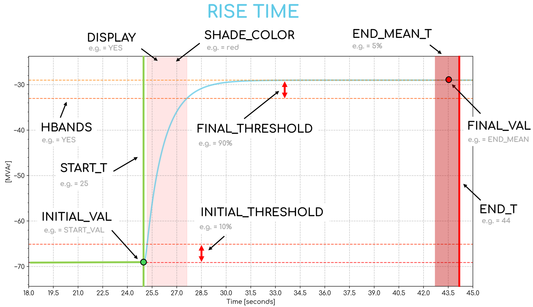
RISE_TIME, START_T=25, END_T=44, INITIAL_VAL=START_VAL, INITIAL_THRESHOLD=10%, FINAL_THRESHOLD=90%, FINAL_VAL=END_MEAN, END_MEAN_T=5%, HBANDS=YES, DISPLAY=YES, SHADE_COLOR=red
Example: Calculate the rise time for each channel on the subplot.
- Begin the calculation at 5 seconds and assume the channels have reached a final value by 5.4 seconds.
- Use the value at 5 seconds as the initial value and the value at 5.4 seconds as the final value.
- Calculate from 10% to 90% of the difference in signal.
RISE_TIME, START_T=5, END_T=5.4, INITIAL_VAL=START_VAL, INITIAL_THRESHOLD=10%, FINAL_VAL=END_VAL, FINAL_THRESHOLD=90%
Example: Calculate the rise time for each channel on the subplot.
- Begin the calculation at 6 seconds and assume the channels have reached a final value by 15 seconds.
- Use the value at 6 seconds as the initial value and the average of the last 5% of the window as the final value. This averaging period is from 14.2 seconds (15 - (15- 6)*5%) to 15 seconds.
- Calculate from 10% to 90% of the difference in signal.
RISE_TIME, START_T=6, END_T=15, INITIAL_VAL=START_VAL, INITIAL_THRESHOLD=10%, FINAL_VAL=END_MEAN, FINAL_THRESHOLD=90%, END_MEAN_T=5%
RECOVERY_T | Recovery time
Also known as 'Pre-disturbance level time'.
RECOVERY_T, START_T=, FAULT_CLEAR_T=, [END_PU=0.95, DISPLAY=YES, NAME=]
Calculates and optionally displays the post-disturbance recovery time for each channel on the subplot.
Arguments:
- RECOVERY_T
- START_T 🔢 (
float): Time the fault or disturbance was applied [seconds]. - FAULT_CLEAR_T 🔢 (
float): Time where the fault or disturbance was cleared [seconds]. - END_PU 🔢 (
float)[Optional]: Per unit threshold of the channel value atSTART_Twhere the signal is considered to have recovered. Defaults to 0.95 (95%). - DISPLAY (
str)[Optional]: Display the recovery time on the subplot. Defaults toDISPLAY=YES. Options:DISPLAY=YES: Recovery time will be displayed on the subplot and in the legend.DISPLAY=NO: Recovery time will not be displayed on the subplot and in the legend.
- HBANDS (
bool)[Optional]: IfYES, adds two dotted horizontal lines corresponding to the value of the signal atSTART_Tand the target recovery value (e.g. the value atSTART_TtimesEND_PU). Defaults toNO(horizontal bands not shown). Only drawn ifDISPLAY=YES. - SHADE_COLOR (
str)[Optional]: Color of the shading. Defaults to a color complementary to the color of the line the calculation was completed on. Options:SHADE_COLOR=: CSS named color, reference the color using the 'Keyword' column here.SHADE_COLOR=RRGGBB: Hexadecimal color code.
- NAME (
str)[Optional]: Output the calculated recovery time as an Internode Variable. Output names must be unique within a Node. - LEGEND (
str)[Optional]: Override the legend label to something other than "Recovery time". E.g. "Pre-disturbance level time".
Example: Calculate the recovery time for each channel on the subplot. Begin the calculation at 5 seconds, the time at which a fault of duration 220 ms is applied. Output the calculated recovery times to an Internode Variable called i_recovery_time. Display the recovery time on the plot.
RECOVERY_T, START_T=5, FAULT_CLEAR_T=5.22, NAME=i_recovery_time
Example Diagram:
The diagram below shows an example RECOVERY_T command.
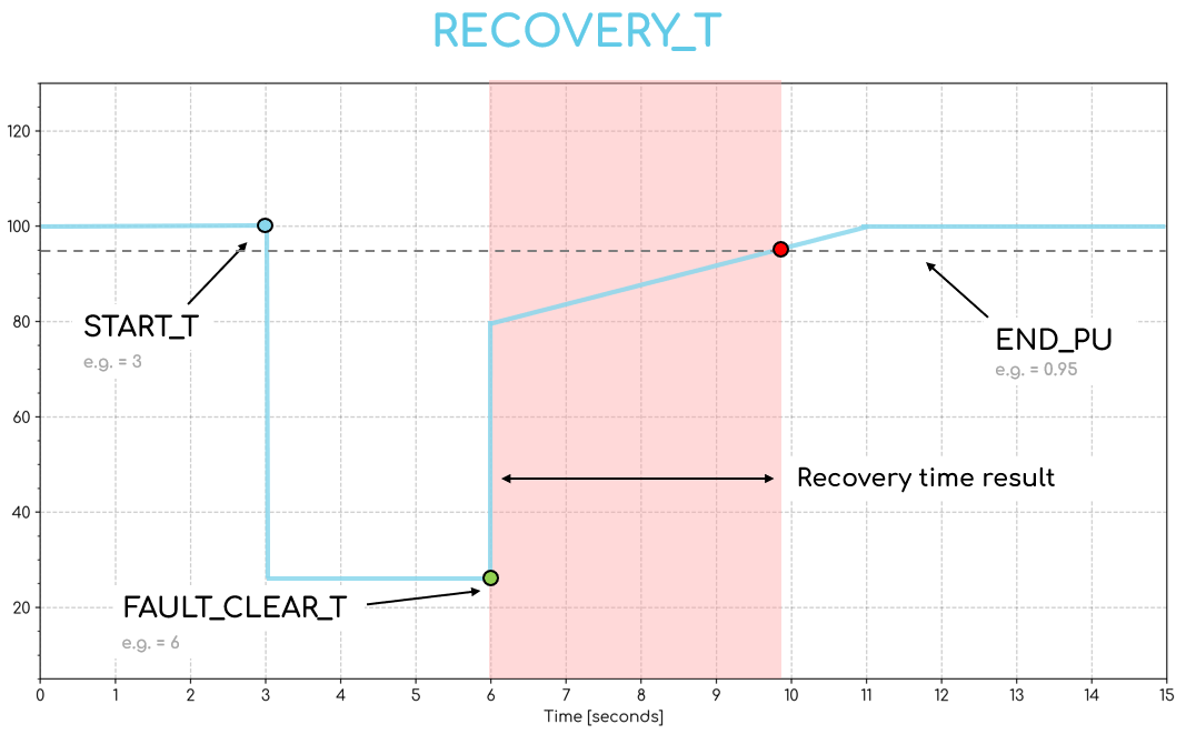
Recovery time calculation example
EDGE | Edge detection
EDGE, TYPE=, [DISPLAY=YES, NAME=]
Outputs the time at which the channel rises to its maximum value or falls to its minimum value.
- This Command is recommended for use with binary signals, such as LVRT or HVRT trigger flags, which toggle between a value of 0 and 1.
Arguments:
- EDGE
- TYPE (
str): The type of edge to detect. Defaults toTYPE=RISING. Options:TYPE=RISING: A rising edge (rising to the maximum value during the simulation).TYPE=FALLING: A falling edge (falling to the minimum value during the simulation).
- DISPLAY (
str)[Optional]: Display the edge detection time on the subplot. Defaults toDISPLAY=YES. Options:DISPLAY=YES: Edge detection time will be displayed on the subplot and in the legend.DISPLAY=NO: Edge detection time will not be displayed on the subplot and in the legend.
- NAME (
str)[Optional]: Output the detected time as an Internode Variable. Output names must be unique within a Node.
Example: Assuming the Internode Variable i_inverter_lvrt is a channel on a subplot, find the time when this channel rises from 0 to its maximum value of 1. Export this time, in seconds, to the Internode Variable i_lvrt_trigger_time:
EDGE, TYPE=RISING, NAME=i_lvrt_trigger_time
COUNT_EDGES | Count edges in a signal
COUNT_EDGES, [START_T=, END_T=, DISPLAY=YES, NAME=]
Counts the number of times a single channel in the subplot toggles between a low value and a high value.
The mid-range of the channel (the average of the maximum and minimum values) is used to determine if a channel transitions between a 'low' and 'high' value.
Arguments:
- COUNT_EDGES
- START_T 🔢 (
float)[Optional]: Start output calculation from this time [seconds]. Defaults to the start of the channel data. - END_T[Optional]: End output calculation at this time [seconds]. Defaults to the end of the channel data. Options:
END_T=x🔢 wherexis afloat: End time isx.END_T=SIM_END: End time is the end of the simulation.
- DISPLAY (
str)[Optional]: IfYES, display the number of edges detected with a dot on the plot. Defaults toDISPLAY=YES. Options:DISPLAY=YES: The number of edges detected will be visible on the subplot (marked by a dot for each transition).DISPLAY=NO: The number of edges will not be visible on the subplot (but the result will appear in the legend).
- NAME (
str)[Optional]: Output the number of edges detected as an Internode Variable. Output names must be unique within a Node.
Example: Assuming the Internode Variable i_inverter_lvrt is a channel on a subplot, count the number of times the i_inverter_lvrt channel transitions from low to high, or high to low. Export this value to the Internode Variable i_num_edges:
COUNT_EDGES, NAME=i_num_edges
OUTPUT | Output single value
OUTPUT, [AT=, VALSCALE=, VAL_FUNCTION=, DISPLAY=YES, NAME=]
Outputs a single value from each channel on the subplot at a specified time.
Arguments:
- OUTPUT
- AT[Optional]: Time in the channel data to extract the value. The extracted value is taken from the first time step after this time [seconds]. Defaults to the end of the channel data. Options:
AT=x🔢 wherexis afloat: At time isx.AT=SIM_END: At time is the end of the simulation.
- VALSCALE 🔢 (
float)[Optional]: Multiplicative scaling factor applied to the output value (i.e. scaled_value = unscaled_value xVALSCALE). Default value is 1. - VAL_FUNCTION 🔢 (
str)[Optional]: Function applied to the output value(s). For example,VAL_FUNCTION=2*VAL+1. Cannot be used in conjunction withVALSCALE. Click here for more information on VAL_FUNCTION syntax and supported functions. - DISPLAY (
str)[Optional]: Display the output value on the subplot. Defaults toDISPLAY=YES. Options:DISPLAY=YES: Output value will be displayed on the subplot and in the legend.DISPLAY=NO: Output value will not be displayed on the subplot and in the legend.
- NAME (
str)[Optional]: Output the single value to an Internode Variable. Output names must be unique within a Node.
Example: Assuming channel i_poc_v is a channel on a subplot, output the value of the channel i_poc_v at the first time step after 5.00 seconds and call this output i_volt_at_start. Do not apply any scaling.
OUTPUT, AT=5, NAME=i_volt_at_start
ADVOUTPUT | Advanced output
ADVOUTPUT, OP=, START_T=, [END_T=, VALSCALE=, VAL_FUNCTION=, DISPLAY=YES, NAME=]
Outputs data from each channel on the subplot with advanced features.
Arguments:
- ADVOUTPUT
- OP (
str): Operation used in the calculation. Options:OP=SUBTRACT: OutputCHANNEL(END_T) - CHANNEL(START_T).OP=ADD: OutputCHANNEL(END_T) + CHANNEL(START_T).OP=MULTIPLY: OutputCHANNEL(END_T) * CHANNEL(START_T).OP=DIVIDE: OutputCHANNEL(END_T) / CHANNEL(START_T).OP=MIN: Output the minimum of the channel betweenSTART_TandEND_T.OP=MAX: Output the maximum of the channel betweenSTART_TandEND_T.OP=MEDIAN: Output the median of the channel betweenSTART_TandEND_T.OP=MEAN: Output the mean of the channel betweenSTART_TtoEND_T.OP=DELTA: Output the difference between the maximum and minimum of the channel betweenSTART_TandEND_T.OP=OVERSHOOT%: Outputs the overshoot percentage. This is the maximum normalized absolute value of the channel betweenSTART_TtoEND_Tdivided by the normalized average of the last 10% of data (e.g.0.9*END_T=toEND_T=)OP=OVERSHOOT%: Overshoot is calculated relative to the change in the signal.
DEPRECATED: The overshoot calculation has been removed fromADVOUTPUT, please use theOVERSHOOTfunction.
- START_T 🔢 (
float): Start output calculation from this time [seconds]. - END_T[Optional]: End output calculation at this time [seconds]. Defaults to the end of the channel data. Options:
END_T=x🔢 wherexis afloat: End time isx.END_T=SIM_END: End time is the end of the simulation.
- VALSCALE 🔢 (
float)[Optional]: Multiplicative scaling factor applied to the output value (i.e. scaled_value = unscaled_value xVALSCALE). Default value is 1. - VAL_FUNCTION 🔢 (
str)[Optional]: Function applied to the output value(s). For example,VAL_FUNCTION=2*VAL+1. Cannot be used in conjunction withVALSCALE. Click here for more information on VAL_FUNCTION syntax and supported functions. - DISPLAY (
str)[Optional]: Display the calculated value on the subplot. Defaults toDISPLAY=YES. Options:DISPLAY=YES: Advanced output value will be displayed on the subplot and in the legend.DISPLAY=NO: Advanced output value will not be displayed on the subplot and in the legend.
- NAME (
str)[Optional]: Output the calculated value to an Internode Variable. Output names must be unique within a Node.
Example: Assuming the Internode Variable i_iq_poc is a channel on a subplot, calculate the difference in reactive current at 5 seconds (pre fault) compared to at 5.43 seconds (during the fault) and export this value as i_delta_iq:
ADVOUTPUT, START_T=5, END_T=5.43, OP=SUBTRACT, NAME=i_delta_iq
ERROR_BAND | Error band
Also known as 'Accuracy bands'.
ERROR_BAND, [START_T=, END_T=, EVENT_AT=, EVENT_AT=], BAND=[], [WINDOW_METHOD=[], CALC=[], DISPLAY=, SHADE_COLOR=, NAME=]
Calculates and displays an error band on the subplot using one channel as a reference. Optionally, outputs the percentage of the samples which appear within the error band.
Arguments:
- ERROR_BAND
- START_T 🔢 (
float)[Optional]: Start the error band from this time [seconds]. Defaults to the start of the channel data. - END_T 🔢 (
float)[Optional]: End the error band at this time [seconds]. Defaults to the end of the channel data. - EVENT_AT 🔢 (
float)[Optional]: Time of the start of an event [seconds]. This time is used in the window method calculation andDELTAmethod. If there are no event times, the transient window will be fromSTART_TtoEND_T. - EVENT_AT 🔢 (
float)[Optional]: Additional event times [seconds]. - BAND (
object): Error band method definition with parameters within square brackets. Multiple methods are supported and can overlap. For overlapping methods, the error band is based on the least restrictive method at any instance. Options:Y 🔢 (
float)[Optional]: Vertical offset of the signal up and down. The offset may be expressed as a value or a percentage [value or %].Example:
BAND=[Y=0.25]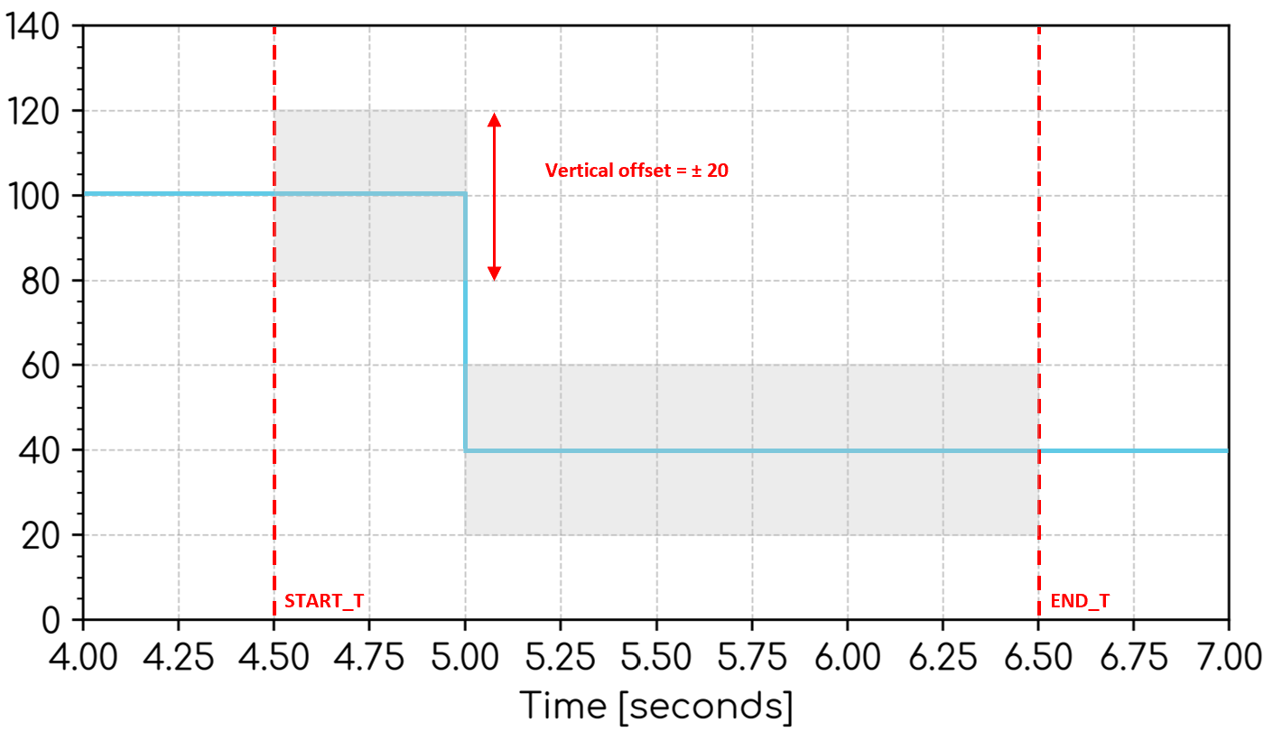
X 🔢 (
float)[Optional]: Horizontal offset of the signal right and left [seconds].Example:
BAND=[X=0.25]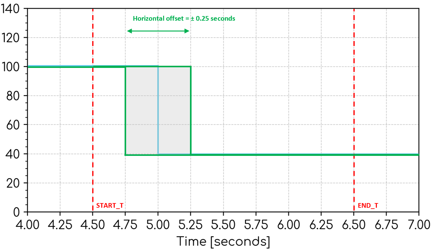
DELTA 🔢 (
float)[Optional]: Vertical offset of the signal up and down. The offset is expressed as a percentage [%] of the difference of the channel values between each event time (i.e. vertical offset = ± `DELTA` \* (value at end of event - value at start of event)). If no event times, then it compares the values at `START_T` and `END_T`. If only one event time, then it compares the values at the event time and `END_T`. If two or more events, then it compares the values between the event time and the next event time or `END_T`.Example:
BAND=[DELTA=10%]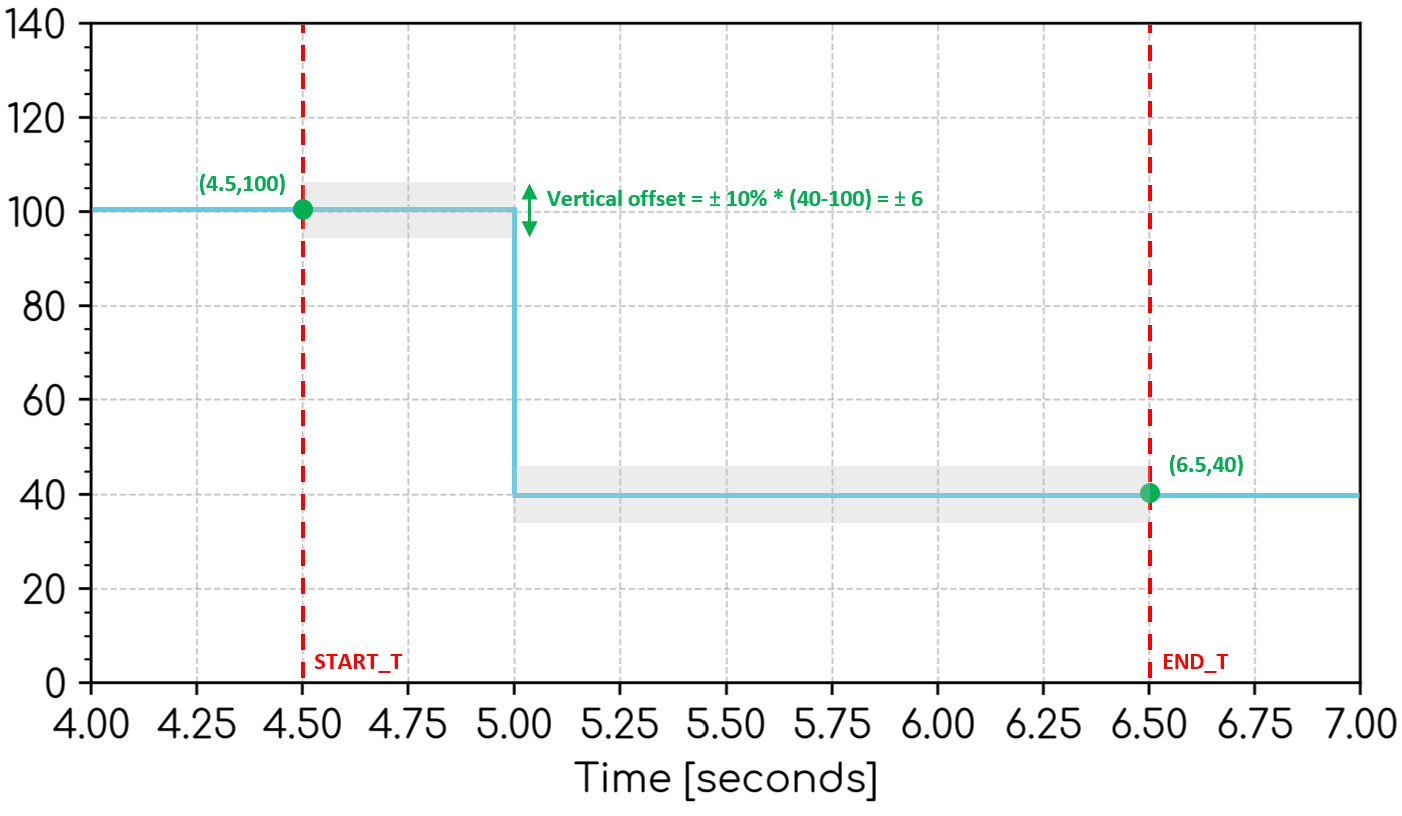
- WINDOW (
str)[Optional]: Location of the error band method definition. Defaults toALL. Options:WINDOW=ALL: Method applies inside transient windows and outside transient windows.WINDOW=IN: Method only applies inside transient windows.WINDOW=OUT: Method only applies outside transient windows.
- BAND (
object)[Optional]: Additional band methods. The overall error band will be the least restrictive of the band arguments specified. - WINDOW_METHOD (
object)[Optional]: Method for determining the end of transient windows between events. Arguments are shared withSETTLING_TIMECommand. The following defaults are chosen.- INITIAL_VAL 🔢 (
float)[Optional]: Default isSTART_VAL. SeeSETTLING_TIMECommand for details. - FINAL_THRESHOLD_OVER 🔢 (
float)[Optional]: Default is 10%. SeeSETTLING_TIMECommand for details. - FINAL_THRESHOLD_UNDER 🔢 (
float)[Optional]: Default is 10%. SeeSETTLING_TIMECommand for details. - FINAL_VAL 🔢 (
float)[Optional]: Default isEND_VAL. SeeSETTLING_TIMECommand for details.
- INITIAL_VAL 🔢 (
- CALC (
object)[Optional]: Options for the error band calculated value. The error band calculation is based on how many data points of the channel fall within the error band around the reference signal. Defaults toCALC=[DISPLAY=NO, WINDOW=ALL].DISPLAY (
str)[Optional]: Display the error band calculation value in the legend. Defaults toDISPLAY=NO. Options:DISPLAY=YES: Error band calculation value will be displayed in the legend.DISPLAY=NO: Error band calculation value will not be displayed in the legend.
Example:
CALC=[DISPLAY=YES]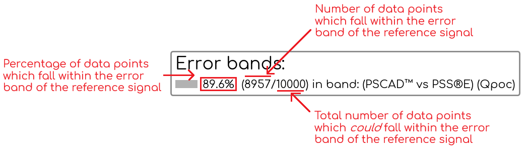
- WINDOW (
str)[Optional]: Choose the region of the channel data to consider for the error band calculation. The calculation region can only be applied where there are existing error bands specified by the BAND= arguments. Defaults toALL. Options:WINDOW=ALL: The error band calculation considers channel values inside the transient window(s) and outside the transient window(s).WINDOW=IN: The error band calculation only considers channel values inside the transient window(s).WINDOW=OUT: The error band calculation only considers channel values outside the transient window(s).
- DISPLAY (
str)[Optional]: Display the error bands on the subplot. Defaults toDISPLAY=YES. If set toNO, the error band calculation will not be displayed even ifCALC=[DISPLAY=YES]is set. Options:DISPLAY=YES: Error bands will be displayed on the subplot.DISPLAY=NO: Error bands will not be displayed on the subplot.
- SHADE_COLOR (
str)[Optional]: Color of the shading. Defaults to your engine's configured default error band color. Options:SHADE_COLOR=: CSS named color, reference the color using the 'Keyword' column here.SHADE_COLOR=RRGGBB: Hexadecimal color code.
- NAME (
str)[Optional]: Outputs the calculated percentage of the channel data which are within the error bands - in accordance with the calculation method, as defined byBANDand the regions, as defined byCALC. Output names must be unique within a Node. - LEGEND (
str)[Optional]: Override the legend label to something other than "Error bands". E.g. "Accuracy bands".
Example: Display an error band on a Qpoc subplot. The error band should be ± 10 MVAr, only between 4 seconds and 8 seconds.
ERROR_BAND, START_T=4, END_T=8, BAND=[Y=10]
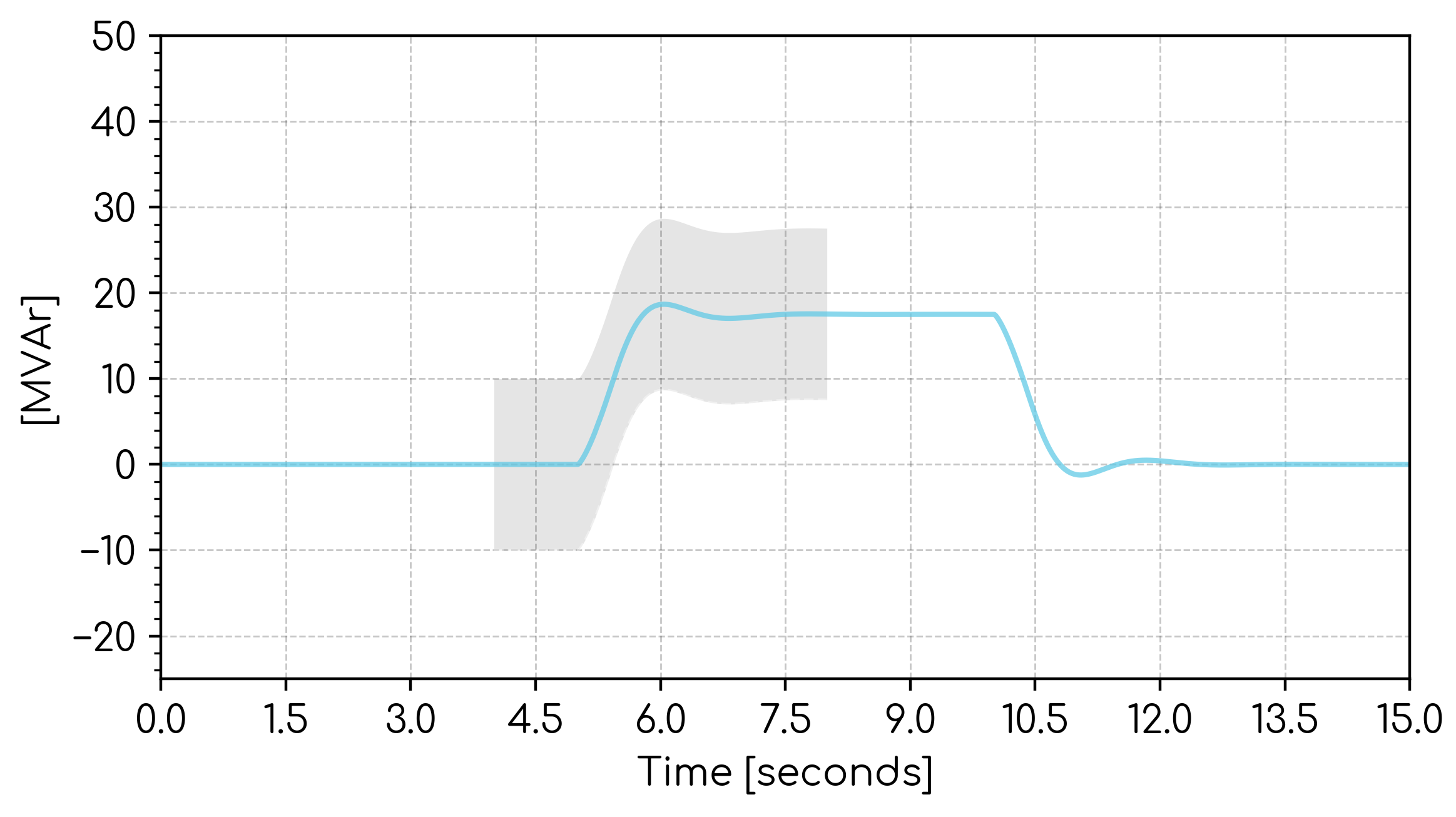
Example: Display an error band on a Qpoc subplot which meets the following requirements:
- There are two transient windows, the first beginning at 5 seconds and the second at 10 seconds. The transient window ends when the final value remains within (final value) ± (FINAL_VAL - INITIAL_VAL)*10%.
- Inside the transient windows, the error band is a vertical offset of the signal up and down. The offset is expressed as a percentage [%] of the difference of the channel values between each event time (i.e. vertical offset = ±
DELTA* (value at end of event - value at start of event)). - Outside the transient windows, the error band is a ±1 MVAr vertical offset of the signal up and down.
- Display a calculation based on how many data points of the channel fall within the error band around the reference signal - only inside the transient windows.
ERROR_BAND, EVENT_AT=5, EVENT_AT=10, BAND=[Y=2, WINDOW=OUT], BAND=[DELTA=10%, WINDOW=IN], CALC=[DISPLAY=YES, WINDOW=IN]
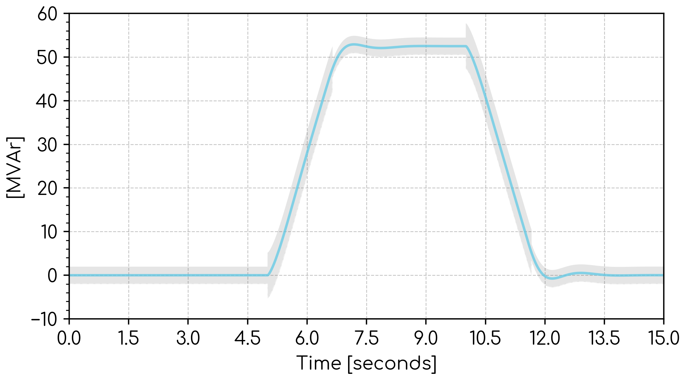
Example: Display an error band on a Qpoc subplot which meets the requirements of Section 6 of AEMO | Power System Model Guidelines | Version 3.0 | 25 September 2025. The following methodology is applied:
- The start of the 'Transient Window' is defined by
EVENT_AT=. The end of the 'Transient Window' is automatically calculated based on when the channel settles to within ±5% of the maximum induced or reference quantity change [Source: Section 6.2 of PSMG]. - Within a Transient Window, the upper and lower error bands are the least restrictive of:
- The channel +10% of the change [Source: Section 6.2.1(b)(i)(A)].
- The channel -10% of the change [Source: Section 6.2.1(b)(i)(A)].
- The channel shifted to the left by 20 milliseconds [Source: Section 6.2.1(b)(i)(B)].
- The channel shifted to the right by 20 milliseconds [Source: Section 6.2.1(b)(i)(B)].
- The channel +2% of the base value provided [Source: Section 6.2.1(d)(i)].
- The channel -2% of the base value provided [Source: Section 6.2.1(d)(i)].
- Outside of a Transient Window, the error bands are bound by:
- Upper bound is +2% of the base value provided [Source: Section 6.2.1(d)(i)].
- Lower bound is -2% of the base value provided [Source: Section 6.2.1(d)(i)].
- Display a calculation based on how many data points of the channel fall within the error band around the reference signal - only inside the transient windows.
ERROR_BAND, EVENT_AT=5, EVENT_AT=10, BAND=[DELTA=10%, WINDOW=IN], BAND=[X=0.02, WINDOW=IN], BAND=[Y=0.02*69.125, WINDOW=ALL], WINDOW_METHOD=[INITIAL_VAL=START_VAL, FINAL_THRESHOLD_OVER=5%, FINAL_THRESHOLD_UNDER=5%, FINAL_VAL=MAX_ABS_OR_END_VAL], CALC=[DISPLAY=YES, WINDOW=IN]
GRADIENT | Gradient of scatter plot
GRADIENT, XMIN=, XMAX=, [INVERT=NO, VALSCALE=, VAL_FUNCTION=, DISPLAY=YES, NAME=]
Calculates the gradient based on least-squares line of best fit for a given range of x-axis values. Horizontal sections (sections of zero or near-zero gradient) are ignored.
Arguments:
- GRADIENT
- XMIN 🔢 (
float): Starting x-axis value to begin calculating the gradient [unit depends on scatter plot units]. - XMAX 🔢 (
float): Ending x-axis value for calculating the gradient [unit depends on scatter plot units]. - INVERT (
bool)[Optional]: IfYES, the calculated gradient will be inverted (i.e. value = 1 / gradient). Defaults toNO. Inversion is applied to unscaled value prior toVALSCALEbeing applied. - VALSCALE 🔢 (
float)[Optional]: Multiplicative scaling factor applied to the output value (i.e. scaled_value = (unscaled_value)INVERT xVALSCALE). Default value is 1. - VAL_FUNCTION 🔢 (
str)[Optional]: Function applied to the output value(s). For example,VAL_FUNCTION=2*VAL+1. Cannot be used in conjunction withVALSCALE. Click here for more information on VAL_FUNCTION syntax and supported functions. - DISPLAY (
str)[Optional]: Display the calculated gradient and line of best fit on the scatter plot. Defaults toDISPLAY=YES. Options:DISPLAY=YES: Gradient and line of best fit will be displayed on the scatter plot.DISPLAY=NO: Gradient and line of best fit will not be displayed on the scatter plot.
- NAME (
str)[Optional]: Outputs the gradient to an Internode Variable. Output names must be unique within a Node.
Example: Calculate the gradient between x=0.9 and x=1.1 and display the gradient and line of best fit on the scatter plot.
GRADIENT, XMIN=0.9, XMAX=1.1
DRAW_LINE | Draw an annotation line on a plot
DRAW_LINE, X1=, X2=, Y1=, Y2=, [TYPE=SOLID, COLOR=black, SHADE_UP=NO, SHADE_DOWN=NO, SHADE_LEFT=NO, SHADE_RIGHT=NO, SHADE_COLOR=black, LEGEND=]
Draws a line segment on the subplot between two specified points, with optional styling and shading. Useful for constructing visual representations of grid code requirements.
Arguments:
- DRAW_LINE
- X1 🔢 (
float): First x-axis data point for line. - Y1 🔢 (
float): First y-axis data point for line. - X2 🔢 (
float): Second x-axis data point for line. - Y2 🔢 (
float): Second y-axis data point for line. - TYPE (
str): The type of line to draw. Defaults toTYPE=SOLID. Options:TYPE=SOLID: A solid line.TYPE=DASHED: A dashed line.
- COLOR (
str)[Optional]: Color of the line. Defaults to black. Line is not visible if the color iswhite. Options:COLOR=: CSS named color, reference the color using the 'Keyword' column here.COLOR=RRGGBB: Hexadecimal color code.
- SHADE_UP / SHADE_DOWN / SHADE_LEFT / SHADE_RIGHT (
bool)[All optional]: Options:=NO: Do not shade in this direction (default).=YES: Shade in this direction infinitely.=z(where z is afloat): Shade the areazunits in this direction.
- SHADE_COLOR (
str)[Optional]: Color of the shading. Defaults to black. Options:SHADE_COLOR=: CSS named color, reference the color using the 'Keyword' column here.SHADE_COLOR=RRGGBB: Hexadecimal color code.
- LEGEND (
str)[Optional]: Legend name for the line segment.DRAW_LINECommands with the sameLEGEND=Argument will be grouped together in the legend.
- Annotations such as lines and shading are not considered when choosing axes limits as part of Auto scaling - only data is considered. If you want to ensure all annotations are shown on a plot, you may need to utilize manual scaling.
- When using Arguments such as
SHADE_DOWN=YES, the shading on the HTML interactive plots will be cropped to prevent shading to infinity.
Example: Draw a red dashed horizontal line across the entire subplot at y = 0.5.
DRAW_LINE, X1=-999, Y1=0.5, X2=999, Y2=0.5, TYPE=DASHED, COLOR=red
Example: Draw a green solid line between (P, Q) = (0, 0.395) and (P, Q) = (1, 0.395)
DRAW_LINE, X1=0, Y1=0.395, X2=1, Y2=0.395, COLOR=green
Example:
- Draw a shaded area to represent the droop characteristic of a solar farm with a maximum reactive power of 80 MVAr, a droop characteristic of 5% and a target voltage of 1.04 p.u. This is a line which intersects (V, Q) = (1.09, -80) and (V, Q) = (0.99, 80).
- Shade +/- 0.5% (0.005 pu on x-axis) around the (invisible) line
DRAW_LINE, X1=0.99, Y1=80, X2=1.09, Y2=-80, COLOR=white, SHADE_LEFT=0.005, SHADE_RIGHT=0.005, SHADE_COLOR=green
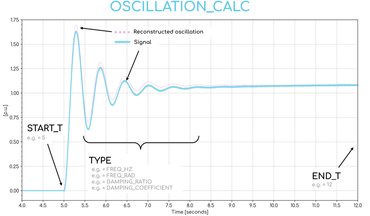
OSCILLATION_CALC | Oscillation calculation
OSCILLATION_CALC, TYPE=, START_T=, [END_T=, VALSCALE=, VAL_FUNCTION=, DISPLAY=], NAME=
Calculates data about an oscillation such as frequency, damping ratio and damping factor.
- The OSCILLATION_CALC command will attempt to identify the dominant mode of oscillation in a signal. This frequency is filtered so that it is sub-synchronous only, e.g. oscillatory frequencies less than or equal to system frequency.
Arguments:
- OSCILLATION_CALC
- TYPE (
str): The type of oscillation calculation to perform. Options:TYPE=FREQ_HZ: Calculate the frequency of the oscillation [Hz].TYPE=FREQ_RAD: Calculate the frequency of the oscillation [Rad/s].TYPE=DAMPING_RATIO: Calculate the damping ratio of the oscillation [Unitless].TYPE=DAMPING_COEFFICIENT: Calculate the damping coefficient of the oscillation [Nepers/s].
- START_T 🔢 (
float): Start of the oscillation window [seconds]. - END_T[Optional]: End of the oscillation window [seconds]. Defaults to the end of the channel data. Options:
END_T=x🔢 wherexis afloat: End time isx.END_T=SIM_END: End time is the end of the simulation.
- VALSCALE 🔢 (
float)[Optional]: Multiplicative scaling factor applied to the output value (i.e. scaled_value = unscaled_value xVALSCALE). Default value is 1. - VAL_FUNCTION 🔢 (
str)[Optional]: Function applied to the output value(s). For example,VAL_FUNCTION=2*VAL+1. Cannot be used in conjunction withVALSCALE. Click here for more information on VAL_FUNCTION syntax and supported functions. - DISPLAY (
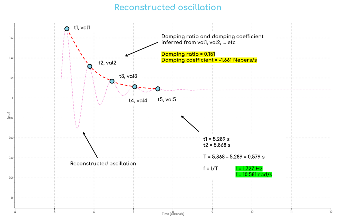
str)[Optional]: Display a reconstructed oscillation using the most impactful frequency. Defaults toDISPLAY=YES. Options:DISPLAY=YES: Reconstructed oscillation will be displayed on the plot.DISPLAY=NO: Reconstructed oscillation will not be displayed on the plot.
- NAME (
str): Output the specified TYPE as an Internode Variable. Output names must be unique within a Node.
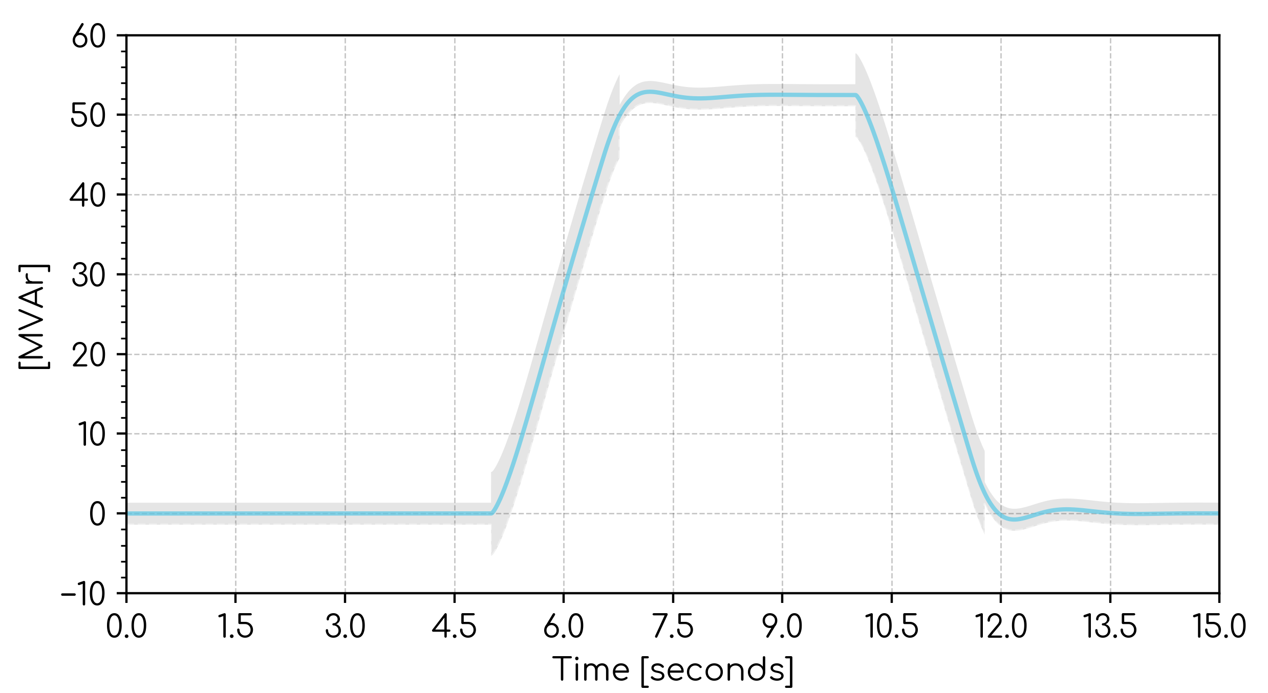
Example Diagram:
The diagrams below show an example OSCILLATION_CALC command.
Example: Calculate the frequency and damping ratio of the oscillation occurring between 5 and 12 seconds and output the result to Internode Variables called i_osc_freq_hz, i_osc_freq_rad, i_osc_damping_ratio and i_osc_damping_coefficient.
OSCILLATION_CALC, TYPE=FREQ_HZ, START_T=5, END_T=12, NAME=i_osc_freq_hz
OSCILLATION_CALC, TYPE=FREQ_RAD, START_T=5, END_T=12, NAME=i_osc_freq_rad
OSCILLATION_CALC, TYPE=DAMPING_RATIO, START_T=5, END_T=12, NAME=i_osc_damping_ratio
OSCILLATION_CALC, TYPE=DAMPING_COEFFICIENT, START_T=5, END_T=12, NAME=i_osc_damping_coefficient
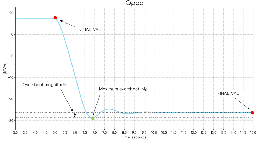
OVERSHOOT | Calculate overshoot
Also known as 'Transient peak'.
OVERSHOOT, [START_T=], [END_T=], CALC_METHOD=, [INITIAL_VAL=], FINAL_VAL=, [END_MEAN_T=, HBANDS=NO, DISPLAY=YES, NAME=]
Calculates and optionally displays the overshoot (and undershoot for negative signal movements) for each channel on the subplot. The calculation can be given as either a percentage or an absolute overshoot value.
Please note that the overshoot calculation is defined as the maximum value of the signal in the direction of the overall signal change. Any initial movement in the opposite direction is not included in the overshoot calculation.
An example of an overshoot is shown below.
 Arguments:
- OVERSHOOT
- START_T 🔢 (
float)[Optional]: Start of the overshoot calculation window [seconds]. Defaults to the start of the channel data. - END_T[Optional]: End of the overshoot calculation window [seconds]. The channel is expected to have reached its final value at this time (e.g. the end of the simulation or just prior to a further disturbance/controlled change). Defaults to the end of the channel data. Options:
END_T=x🔢 wherexis afloat: End time isx.END_T=SIM_END: End time is the end of the simulation.
- CALC_METHOD (
str): There are three definitions for how overshoot is calculated. The calculation methodology can differ between grid codes. In the overshoot calculation methods, only the denominator changes; the numerator stays the same.PERCENT_DELTA: Overshoot is calculated relative to the change in the signal.
CALC_METHOD=PERCENT_DELTAThe overshoot is defined as the maximum system output minus the final settled value, divided by the actual change in system output (i.e., from its initial value to the final settled value), when the final settled value is within the defined settling band, expressed as a percentage.
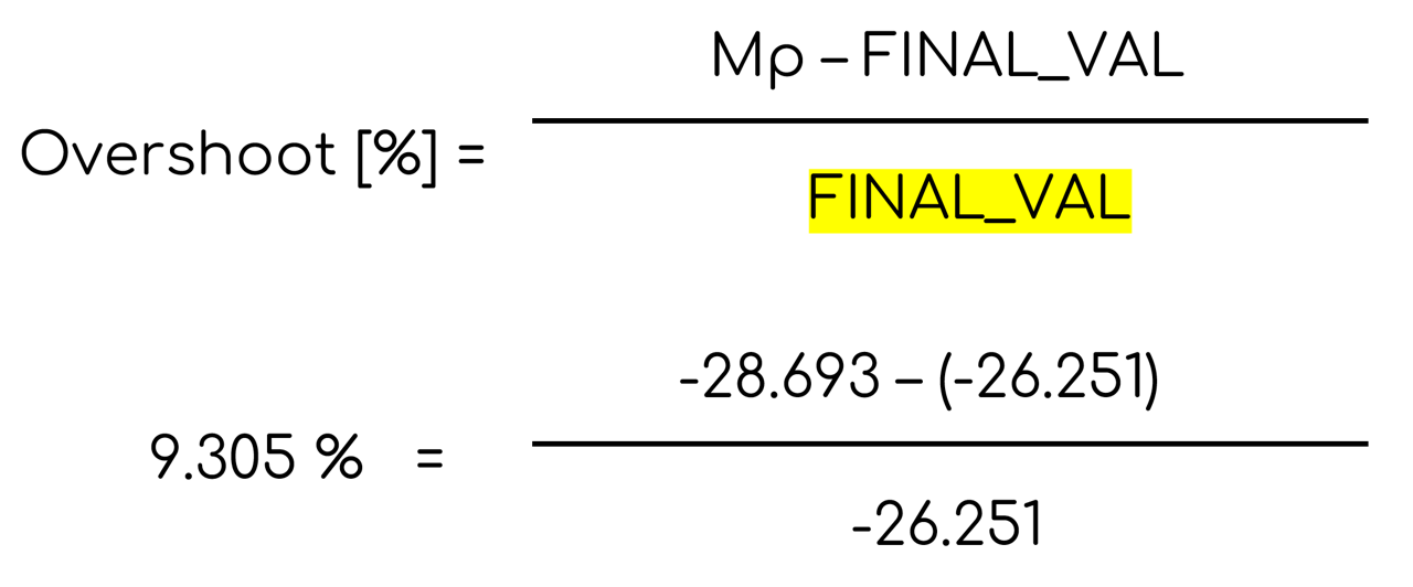
PERCENT_FINAL_VAL: Overshoot is calculated relative to final value only.
CALC_METHOD=PERCENT_FINAL_VALThe overshoot is defined as the maximum amount the system overshoots its final value divided by its final value. This definition does not take into account the step change (i.e. initial value). It is also limited when the final value approaches zero, because the overshoot calculation can grow considerably when it requires division by a value approaching zero.
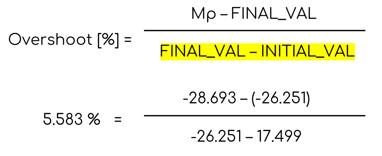
ABSOLUTE: Overshoot is calculated as the absolute difference between the peak value and the final value, expressed in the units of the measured signal.
CALC_METHOD=ABSOLUTEOvershoot is calculated as the absolute difference between the peak value (Mp) and the final value, expressed in the units of the measured signal. The calculation method is the same as the other approaches, except that it uses only the numerator of the formula. This method can be used to calculate the overshoot magnitude in the units of the signal.

- INITIAL_VAL[Optional]: Used if
CALC_METHOD=PERCENT_DELTA. Initial channel value used in the overshoot calculations. Options:INITIAL_VAL=x🔢 wherexis afloat: Initial value isx.INITIAL_VAL=START_VAL: Initial value is the channel value atSTART_T.
- FINAL_VAL: Final channel value used in overshoot calculations. Options:
FINAL_VAL=x🔢 wherexis afloat: Final value isx.FINAL_VAL=END_VAL: Final value is the channel value atEND_T.FINAL_VAL=END_MEAN: Final value is the average of the values from (END_T-END_MEAN_T) to (END_T).
- END_MEAN_T (
float %)[Optional]: Used ifFINAL_VAL=END_MEAN. The time prior toEND_Tused in the average calculation. When specified as a percentage, the time is END_MEAN_T% * (END_T-START_T). - HBANDS (
bool)[Optional]: IfYES, adds dotted horizontal lines corresponding to the values used in the overshoot calculation, e.g.INITIAL_VAL,OVERSHOOT_VAL,FINAL_VAL. Defaults toNO(horizontal bands not shown). Only drawn ifDISPLAY=YES.INITIAL_VALis shown only whenCALC_METHOD=PERCENT_DELTA, as this is the only method that usesINITIAL_VAL - DISPLAY (
str)[Optional]: Display the overshoot on the subplot and in the legend. Defaults toDISPLAY=YES. Options:DISPLAY=YES: Overshoot will be displayed on the subplot and in the legend.DISPLAY=NO: Overshoot will not be displayed on the subplot and in the legend.
- NAME (
str)[Optional]: Output the calculated overshoot as an Internode Variable. Output names must be unique within a Node. - LEGEND (
str)[Optional]: Override the legend label to something other than "Overshoot". E.g. "Transient peak".
Example: Calculate the overshoot for each channel on the subplot.
- Begin the calculation at 5 seconds and assume the channels have reached a final value by 15 seconds.
- Use the value at 5 seconds as the initial value and the value at 15 seconds as the final value.
- Calculates the overshoot relative to the change in the signal, expressed in %.
OVERSHOOT, START_T=5, END_T=15, CALC_METHOD=PERCENT_DELTA, INITIAL_VAL=START_VAL, FINAL_VAL=END_VAL, HBANDS=YES, DISPLAY=YES
Advanced Parameters
pf.axis.enabled
- Description: Enabled by default. If
No, any power factor subplots will be displayed with a regular axis. - Type:
str - Units: N/A
- Default: Yes
- Range: Yes or No
pf.axis.enabled=No
Deprecated Commands
The following commands are no longer recommended for new Projects as they have been replaced with new commands with expanded functionality.
STYLE | Style scatter plot
STYLE, TYPE=
Applies a pre-built style to a scatter plot.
STYLE, TYPE= command is no longer recommended for new Projects. Instead, use the DRAW_LINE Command.
Note that the following commands are equivalent:
STYLE, TYPE=5255IQ
// Quadrant 1
DRAW_LINE, X1=1.1, Y1=0, X2=999, Y2=0, COLOR=white, SHADE_UP=YES, SHADE_COLOR=grey
// Quadrant 2
DRAW_LINE, X1=0.0, Y1=1.0, X2=0.6, Y2=1.0, COLOR=white, SHADE_UP=YES, SHADE_COLOR=green
DRAW_LINE, X1=0.6, Y1=1.0, X2=0.85, Y2=0, COLOR=white, SHADE_UP=YES, SHADE_COLOR=green
DRAW_LINE, X1=0.85, Y1=0, X2=0.9, Y2=0, COLOR=white, SHADE_UP=YES, SHADE_COLOR=green
// Quadrant 3
DRAW_LINE, X1=-999, Y1=0, X2=0.9, Y2=0, COLOR=white, SHADE_DOWN=YES, SHADE_COLOR=grey
// Quadrant 4
DRAW_LINE, X1=1.1, Y1=0, X2=1.15, Y2=0, COLOR=white, SHADE_DOWN=YES, SHADE_COLOR=green
DRAW_LINE, X1=1.15, Y1=0, X2=2, Y2=-5.1, COLOR=white, SHADE_DOWN=YES, SHADE_COLOR=green

// Axes lines
DRAW_LINE, X1=1, Y1=-999, X2=1, Y2=999, COLOR=black
DRAW_LINE, X1=-999, Y1=0, X2=999, Y2=0, COLOR=black
Note that the following commands are equivalent:
STYLE, TYPE=52511
// Quadrant 1
DRAW_LINE, X1=50, Y1=0, X2=999, Y2=0, COLOR=white, SHADE_UP=YES, SHADE_COLOR=grey
// Quadrant 3
DRAW_LINE, X1=-999, Y1=0, X2=50, Y2=0, COLOR=white, SHADE_DOWN=YES, SHADE_COLOR=grey

// Axes lines
DRAW_LINE, X1=-999, Y1=0, X2=999, Y2=0, COLOR=black
DRAW_LINE, X1=50, Y1=-999, X2=50, Y2=999, COLOR=black
Note that the following commands are equivalent:
STYLE, TYPE=52513
DRAW_LINE, X1=-999, Y1=0, X2=999, Y2=0, COLOR=black
DRAW_LINE, X1=1, Y1=-999, X2=1, Y2=999, COLOR=black
Arguments:
- STYLE
- TYPE (
str): Style type. Options:TYPE=5255IQ: Used for Australian NER S5.2.5.5 FRT iq injection studies. Centers the x-axis around V = 1 [p.u.] and the y-axis around Iq = 0 A [p.u.]. Sets axis label precision to 2 decimal places. Adds two shaded areas which correspond with the Automatic Access Standard (AAS) and Minimum Access Standard (MAS) as per S5.2.5.5 of the Australian NER.TYPE=52511: Used for Australian NER S5.2.5.11 frequency control studies. Centers the x-axis around f= 50 [Hz] and the y-axis around P = 0 [MW]. Sets axis label precision to 0 decimal places. Adds two shaded areas which correspond with the Automatic Access Standard (AAS) as per S5.2.5.11 of the Australian NER.TYPE=52513: Used for Australian NER S5.2.5.13 voltage droop characteristic studies. Centers the x-axis around V = 1 [p.u.] and the y-axis around Q = 0 [MVAr]. Overrides the x-axis limit to between V = 0.9 [p.u.] and V = 1.1 [p.u.]. Sets axis label precision to 2 decimal places.
Example: Apply Australian NER S5.2.5.13 styling to a scatter plot of a Q(V) droop curve.
STYLE, TYPE=52513
This Command may override manual x-axis/y-axis scaling.
RISE_T | Rise time
RISE_T, START_T=, [END_T=, START_PU=0.1, END_PU=0.9, HBANDS=NO, DISPLAY=YES, NAME=]
RISE_T command is no longer recommended for new Projects. Instead, use the RISE_TIME Command. Note that the following commands are equivalent:
RISE_T, START_T=5, END_T=5.1, START_PU=0.1, END_PU=0.9
RISE_TIME, START_T=5, END_T=5.1, INITIAL_VAL=START_VAL, INITIAL_THRESHOLD=10%, FINAL_THRESHOLD=90%, FINAL_VAL=END_VAL
Calculates and optionally displays the rise time for each channel on the subplot.
Arguments:
- RISE_T
- START_T 🔢 (
float): Start rise time calculation from this time [seconds]. - END_T 🔢 (
float)[Optional]: A time by which the channel is expected to have reached its final value (e.g. the end of the simulation or just prior to a further disturbance/controlled change) [seconds]. Defaults to the end of the channel data. - START_PU 🔢 (
float)[Optional]: Per unit threshold of the value atEND_Twhere the rise time calculation starts. Defaults to 0.1 (10%). - END_PU 🔢 (
float)[Optional]: Per unit threshold of the value atEND_Twhere the signal is considered 'risen'. Defaults to 0.9 (90%). - HBANDS (
bool)[Optional]: IfYES, adds dotted horizontal lines corresponding to theEND_PUthreshold bands to visually show the acceptable settling band. Defaults toNO(horizontal bands not shown). Only drawn ifDISPLAY=YES. - DISPLAY (
str)[Optional]: Display the rise time on the subplot. Defaults toDISPLAY=YES. Options:DISPLAY=YES: Rise time will be displayed on the subplot and in the legend.DISPLAY=NO: Rise time will not be displayed on the subplot and in the legend.
- SHADE_COLOR (
str)[Optional]: Color of the shading. Defaults to a color complementary to the color of the line the calculation was completed on. Options:SHADE_COLOR=: CSS named color, reference the color using the 'Keyword' column here.SHADE_COLOR=RRGGBB: Hexadecimal color code.
- NAME (
str)[Optional]: Output the calculated rise time as an Internode Variable. Output names must be unique within a Node.
Example: Calculate the rise time for each channel on the subplot. Begin the calculation at 5 seconds and assume the channels have settled by 5.1 seconds. Do not output to an Internode Variable. Display the rise time on the subplot.
RISE_T, START_T=5, END_T=5.1
Rise time calculation example
Notes on the interpretation of "maximum change induced in that quantity" in Chapter 10 of AEMC | National Electricity Rules | Version 222 | 19 December 2024
Rise time is defined in Chapter 10 of the NER [1] as the following:
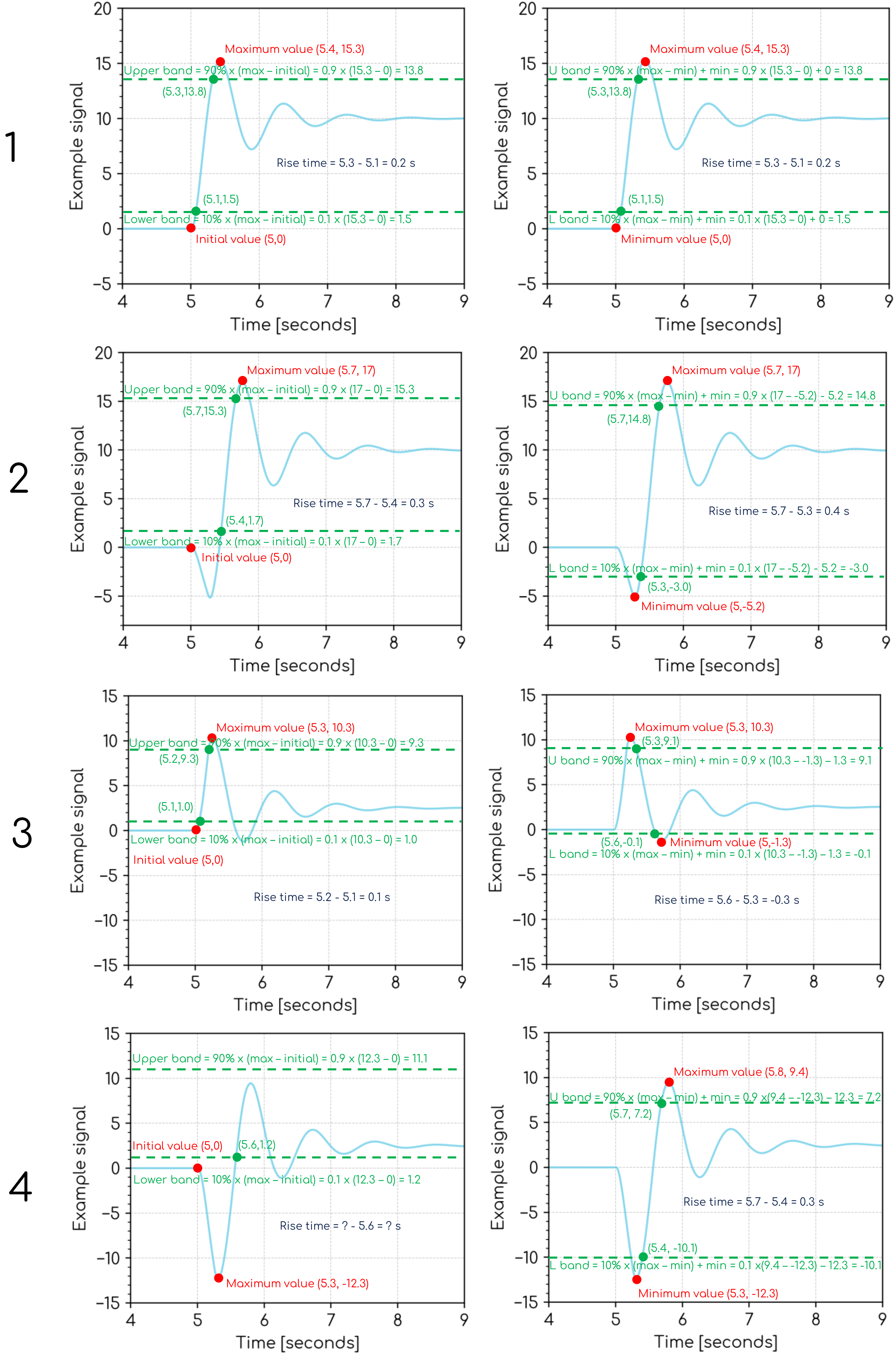
In relation to a control system, the time taken for an output quantity to rise from 10% to 90% of the maximum change induced in that quantity by a step change of an input quantity.
However, this definition is subjective due to the lack of definition of the term "maximum change induced in that quantity". AEMO has described the NER as having, "...an unusual definition of rise time...where it is more usual to describe the rise time in terms of 10% - 90% of the sustained change." [2]. The following note details gridmo's interpretation of this subjective definition.
There are two potential interpretations of "maximum change induced in that quantity":
- [gridmo interpretation] The maximum change in signal when compared to the initial value prior to the event.
- The maximum minus the minimum of the signal across the entire duration of the event.
We note that the proposed AEMC rule change ERC0393 [3] is proposing to amend the definition of rise time to remove the subjective definition, "maximum change induced in that quantity".
COMMENCEMENT_T | Commencement time
COMMENCEMENT_T, START_T=, [END_T=, START_PU=0, END_PU=0.1, HBANDS=NO, DISPLAY=YES, NAME=]
Calculates commencement time for each channel on the subplot.
COMMENCEMENT_T command is no longer recommended for new Projects. Instead, use the RISE_TIME Command.
Arguments:
- COMMENCEMENT_T
- START_T 🔢 (
float): Start commencement time calculation from this time [seconds]. - END_T 🔢 (
float)[Optional]: A time by which the channel is expected to have reached its final value (e.g. the end of the simulation or just prior to a further disturbance/controlled change) [seconds]. Defaults to the end of the channel data. - START_PU 🔢 (
float)[Optional]: Per unit threshold of the value atEND_Twhere the commencement time calculation starts. Defaults to 0 (0%). - END_PU 🔢 (
float)[Optional]: Per unit threshold of the value atEND_Twhere the signal has settled. Defaults to 0.1 (10%). - HBANDS (
bool)[Optional]: IfYES, adds dotted horizontal lines corresponding to theEND_PUthreshold. Defaults toNO(horizontal bands not shown). Only drawn ifDISPLAY=YES. - DISPLAY (
str)[Optional]: Display the commencement time on the subplot. Defaults toDISPLAY=YES. Options:DISPLAY=YES: Commencement time will be displayed on the subplot and in the legend.DISPLAY=NO: Commencement time will not be displayed on the subplot and in the legend.
- SHADE_COLOR (
str)[Optional]: Color of the shading. Defaults to a color complementary to the color of the line the calculation was completed on. Options:SHADE_COLOR=: CSS named color, reference the color using the 'Keyword' column here.SHADE_COLOR=RRGGBB: Hexadecimal color code.
- NAME (
str)[Optional]: Output the calculated commencement time as an Internode Variable. Output names must be unique within a Node.
Example: Calculate the commencement time for each channel on the subplot. Begin the calculation at 5 seconds and assume the channels have settled by 5.1 seconds. Do not output to an Internode Variable. Display the commencement time on the subplot.
COMMENCEMENT_T, START_T=5, END_T=5.1
SETTLE_T | Settling time
SETTLE_T, START_T=, [END_T=, END_PU=0.1, HBANDS=NO, DISPLAY=YES, NAME=]
SETTLE_T command is no longer recommended for new Projects. Instead, use the SETTLING_TIME Command. Note that the following commands are equivalent:
SETTLE_T, START_T=5, END_T=15, END_PU=0.1
SETTLING_TIME, START_T=5, END_T=15, INITIAL_VAL=START_VAL, FINAL_THRESHOLD_OVER=10%, FINAL_THRESHOLD_UNDER=10%, FINAL_VAL=MAX_ABS_OR_END_VAL
Calculates and optionally displays the settling time for each channel on the subplot.
Arguments:
- SETTLE_T
- START_T 🔢 (
float): Start settling time calculation from this time [seconds]. - END_T 🔢 (
float)[Optional]: A time by which the channel is expected to have reached its final value (e.g. the end of the simulation or just prior to a further disturbance/controlled change) [seconds]. Defaults to the end of the channel data. - END_PU 🔢 (
float)[Optional]: Per unit threshold of the value atEND_Twhere the signal is considered settled (if the signal remains within ± this multiplier of the final value). Defaults to 0.1 (10%). - HBANDS (
bool)[Optional]: IfYES, adds dotted horizontal lines corresponding to theEND_PUthreshold bands to visually show the acceptable settling band. Defaults toNO(horizontal bands not shown). Only drawn ifDISPLAY=YES. - DISPLAY (
str)[Optional]: Display the settling time on the subplot. Defaults toDISPLAY=YES. Options:DISPLAY=YES: Settling time will be displayed on the subplot and in the legend.DISPLAY=NO: Settling time will not be displayed on the subplot and in the legend.
- SHADE_COLOR (
str)[Optional]: Color of the shading. Defaults to a color complementary to the color of the line the calculation was completed on. Options:SHADE_COLOR=: CSS named color, reference the color using the 'Keyword' column here.SHADE_COLOR=RRGGBB: Hexadecimal color code.
- NAME (
str)[Optional]: Output the calculated settling time as an Internode Variable. Output names must be unique within a Node.
Example: Calculate the settling time for each channel on the subplot. Begin the calculation at 5 seconds and assume the channels have settled by 15 seconds. Output the calculated settling times to an Internode Variable called i_settling_time. Do not display the settling time on the subplot.
SETTLE_T, START_T=5, END_T=15, DISPLAY=NO, NAME=i_settling_time
Settling time calculation examples
- No overshoot
- Significant overshoot
- Oscillation
Notes on the interpretation of "maximum change in that output quantity" in Chapter 10 of AEMC | National Electricity Rules | Version 222 | 19 December 2024
Settling time is defined in Chapter 10 of the NER [1] as the following:
In relation to a control system, the time measured from initiation of a step change in an input quantity to the time when the magnitude of error between the output quantity and its final settling value remains less than 10% of:
- if the sustained change in the quantity is less than half of the maximum change in that output quantity, the maximum change induced in that output quantity; or
- the sustained change induced in that output quantity.
However, this definition is subjective due to the lack of definition of the term "maximum change in that output quantity". AEMO has described the NER as having, "...non-standard definition of settling time." [2]. The following note details gridmo's interpretation of this subjective definition.
There are two potential interpretations of "maximum change in that output quantity":
- [gridmo interpretation] The maximum change in signal when compared to the initial value prior to the event.
- The maximum minus the minimum of the signal across the entire duration of the event.
We note that the proposed AEMC rule change ERC0393 [3] is proposing to amend the definition of settling time to remove the subjective definition, "maximum change in that output quantity".
SIMPLEBANDS | Simple error bands
SIMPLEBANDS, [BANDWIDTH=3%, DISPLAY=NO, BAND_START_T=, BAND_END_T=, NAME=]
SIMPLEBANDS command is no longer recommended for new Projects. Instead, use the ERROR_BAND Command. Note that the following commands are equivalent:
SIMPLEBANDS, BANDWIDTH=2
ERROR_BAND, BAND=[Y=2]
Calculates and displays simple offset-based or percentage-based symmetrical error bands on the subplot using one channel as a reference.
Arguments:
- SIMPLEBANDS
- BANDWIDTH 🔢 (
float)[Optional]: Vertical width of error bands. Defaults toBANDWIDTH=3%. Options:BANDWIDTH=X: Absolute value offset to apply to the error bands. error_bands = reference_value ± X.BANDWIDTH=X%: Relative multiplicative scale to apply to the error bands. error_bands = reference_value × (1 ± X%).
- DISPLAY (
str)[Optional]: Display the calculated percentage of the samples which appear within the error band bounds on the subplot. This Argument doesn't affect whether the error bands are displayed on the subplot. Defaults toDISPLAY=NO. Options:DISPLAY=YES: Percentage will be displayed in the legend.DISPLAY=NO: Percentage will not be displayed in the legend.
- SHADE_COLOR (
str)[Optional]: Color of the shading. Defaults to your engine's configured default error band color. Options:SHADE_COLOR=: CSS named color, reference the color using the 'Keyword' column here.SHADE_COLOR=RRGGBB: Hexadecimal color code.
- BAND_START_T 🔢 (
float)[Optional]: Start the error band on the plot from this time [seconds]. Defaults to the start of the channel data. - BAND_END_T: End the error band on the plot at this time [seconds]. Defaults to the end of the channel data. Options:
BAND_END_T=x🔢 wherexis afloat: Band end time isx.BAND_END_T=SIM_END: Band end time is the end of the simulation.
- NAME (
str)[Optional]: Outputs the percentage of the samples which appear within the error band bounds to an Internode Variable. The percentage of data points within the error bands is calculated only for the period betweenBAND_START_T=andBAND_END_T=. Output names must be unique within a Node.
Example: Display error bands on the active power subplot with an absolute offset of ± 10 MW.
SIMPLEBANDS, BANDWIDTH=10
Example: Display error bands +/- 2 MVAr on the reactive power subplot, only between 10 seconds and 20 seconds.
SIMPLEBANDS, BANDWIDTH=2, BAND_START_T=10, BAND_END_T=20
DELTA_ERRORBANDS | Error bands calculated by the change in a channel
DELTA_ERRORBANDS, [START_T=, END_T=, BANDWIDTH=10%, DISPLAY=NO, BAND_START_T=, BAND_END_T=, NAME=]
DELTA_ERRORBANDS command is no longer recommended for new Projects. Instead, use the ERROR_BAND Command. Note that the following commands are equivalent:
DELTA_ERRORBANDS, START_T=5, END_T=10, BANDWIDTH=10%
ERROR_BAND, START_T=5, END_T=10, BAND=[DELTA=10%]
Calculates and displays error bands based on an absolute difference between a channel calculated at two times, using that channel as a reference, with a scale factor. Specifically, the error band's width is equal to the absolute value of the change in the channel between the channel at START_T and the channel at END_T, multiplied by the BANDWIDTH factor.
Arguments:
- DELTA_ERRORBANDS
- START_T 🔢 (
float)[Optional]: Initial time to calculate change in channel from [seconds]. Defaults to the start of the channel. - END_T: End time for the change in channel [seconds]. Defaults to the end of the channel. Options:
END_T=x🔢 wherexis afloat: End time isx.END_T=SIM_END: End time is the end of the simulation.
- BANDWIDTH 🔢 (
float%)[Optional]: Scale to apply to the error band vertical width. Defaults to10%. - DISPLAY (
str)[Optional]: Display the calculated percentage of the samples which appear within the error band bounds on the subplot. This Argument doesn't affect whether the error bands are displayed on the subplot. Defaults toDISPLAY=NO. Options:DISPLAY=YES: Percentage will be displayed in the legend.DISPLAY=NO: Percentage will not be displayed in the legend.
- SHADE_COLOR (
str)[Optional]: Color of the shading. Defaults to your engine's configured default error band color. Options:SHADE_COLOR=: CSS named color, reference the color using the 'Keyword' column here.SHADE_COLOR=RRGGBB: Hexadecimal color code.
- BAND_START_T 🔢 (
float)[Optional]: Start the error band on the plot from this time [seconds]. Defaults to the start of the channel data. - BAND_END_T: End the error band on the plot at this time [seconds]. Defaults to the end of the channel data. Options:
BAND_END_T=x🔢 wherexis afloat: Band end time isx.BAND_END_T=SIM_END: Band end time is the end of the simulation.
- NAME (
str)[Optional]: Outputs the percentage of the samples which appear within the error band bounds to an Internode Variable. The percentage of data points within the error bands is calculated only for the period betweenBAND_START_T=andBAND_END_T=. Output names must be unique within a Node.
Example: Display error bands on the subplot based on the change in active power between 5 seconds and 10 seconds. Use the default BANDWIDTH of 10%. The applied error bands will be equal to the absolute value of the change in the channel on this subplot between 5 seconds and 10 seconds, multiplied by 10%.
DELTA_ERRORBANDS, START_T=5, END_T=10
Example: Display error bands on the subplot only between 15 seconds and 22 seconds. Set the error band width to 5% of the change in the channel between 5 seconds and 30 seconds.
DELTA_ERRORBANDS, START_T=5, END_T=30, BANDWIDTH=5%, BAND_START_T=15, BAND_END_T=22
ADVBANDS | Advanced error bands
ADVBANDS, BASE=, [TAT=, TAT=, DISPLAY=NO, NAME=]
ADVBANDS command is no longer recommended for new Projects. Instead, use the ERROR_BAND Command. Note that the following commands are 'almost' equivalent:
ADVBANDS, BASE=40, TAT=10, TAT=20
ERROR_BAND, EVENT_AT=10, EVENT_AT=20, BAND=[Y=0.02*40, WINDOW=ALL], BAND=[Y=0.02, WINDOW=IN], BAND=[DELTA=10%, WINDOW=IN]
NOTE: For underdamped signals, the transient window calculation in ADVBANDS will be slightly different since it considers the "maximum induced" change rather than "sustained change".
Calculates and displays advanced error bands on the subplot using one channel as a reference. Advanced error bands are used to meet specific grid code requirements. Optionally, outputs the percentage of the samples which appear within the error band bounds.
Arguments:
- ADVBANDS
- BASE 🔢 (
float): Base value to use for the error band calculation. - TAT 🔢 (
float)[Optional][Multiple]: Time of the start of a transient, where different error band calculation methodology may be required. Defaults to no transients. Multiple Arguments supported. - DISPLAY (
str)[Optional]: Display the calculated percentage of the samples which appear within the error band bounds on the subplot. This Argument doesn't affect whether the error bands are displayed on the subplot. Defaults toDISPLAY=NO. Options:DISPLAY=YES: Percentage will be displayed in the legend.DISPLAY=NO: Percentage will not be displayed in the legend.
- SHADE_COLOR (
str)[Optional]: Color of the shading. Defaults to your engine's configured default error band color. Options:SHADE_COLOR=: CSS named color, reference the color using the 'Keyword' column here.SHADE_COLOR=RRGGBB: Hexadecimal color code.
- NAME (
str)[Optional]: Outputs the percentage of the samples which appear within the error band transient window bounds to an Internode Variable. Output names must be unique within a Node.
Currently, ADVBANDS only supports error bands derived in accordance with Section 6 of AEMO | Power System Model Guidelines | Version 2 | July 2023. The following methodology is applied:
- The start of the 'Transient Window' is defined by the user using
TAT=. - The end of the 'Transient Window' is automatically calculated based on when the channel settles to within ±5% of the maximum induced or reference quantity change [Source: Section 6.2 of PSMG].
- Within a Transient Window, the upper and lower error bands are the least restrictive of:
- The channel +10% of the maximum induced or reference quantity change [Source: Section 6.2.1(b)(i)(A)].
- The channel -10% of the maximum induced or reference quantity change [Source: Section 6.2.1(b)(i)(A)].
- The channel shifted to the left by 20 milliseconds [Source: Section 6.2.1(b)(i)(B)].
- The channel shifted to the right by 20 milliseconds [Source: Section 6.2.1(b)(i)(B)].
- The channel +2% of the
BASE=value provided [Source: Section 6.2.1(d)(i)]. - The channel -2% of the
BASE=value provided [Source: Section 6.2.1(d)(i)].
- Outside of a Transient Window, the error bands are bound by:
- Upper bound is +2% of the
BASE=value provided [Source: Section 6.2.1(d)(i)]. - Lower bound is -2% of the
BASE=value provided [Source: Section 6.2.1(d)(i)].
- Upper bound is +2% of the
The BASE= values should be chosen using the following logic:
- If the channel is active power, then
BASE=should be your project's registered capacity [MW]. - If the channel is reactive power, then
BASE=should be your project's maximum reactive power [MVAr]. - If the channel is voltage, then
BASE=should be 1.
Example: Display error bands compliant with AEMO's Power System Modelling Guidelines on the reactive power subplot. Use a base of 40 MVAr. The channel should have two Transient Windows starting at 10 seconds and 20 seconds.
ADVBANDS, BASE=40, TAT=10, TAT=20