How to model complex power system faults

Background

Commonly, once single machine infinite bus (SMIB) tests are completed, the model of a generating system is merged into a wide-area dynamic network model to investigate the generating system's response when connected to other generation.

As part of these studies, complex network faults are often simulated to test the generating system's response to various network disturbances.

In this example we will show you how to model complex network faults such as auto-reclose, control trips, run-backs and intertrips using gridmo.

Event type	Description
Auto-reclose (ARC)	A fault is applied to a network asset (usually an overhead line), the line is tripped and then automatically closes back into service after a fixed delay. This is because the fault may no longer be present, such as a tree branch which fell onto a line but then fell off shortly afterwards. Multiple reclose attempts can be made before the line 'locks-out' (is disconnected pending human intervention)
Control trip	A network asset is disconnected when a fault is not present, equivalent to a control room operator manually disconnecting a line.
Run-back scheme	A network asset is disconnected (either with or without a fault) which triggers a special protection scheme. This system instructs one or more generator(s) to 'run-back' their active power to a predefined level, which may be 0 MW. Generators which have been run-back still provide voltage support (they are not disconnected). Typically used to prevent thermal overloads on network assets.
Intertrip scheme	A network asset is disconnected (either with or without a fault) which triggers a special protection scheme. This system instructs one or more generator(s) to immediately disconnect from the network. Typically used to prevent grid-following generating systems from operating in a network with insufficient fault level (system strength).

tip

You can download the complete example project file used in this tutorial from the below link. The example data file and the models required to run this example simulation are packaged with the gridmo Engine - no further configuration is required.

Note there are additional faults in the downloadable example file (above) which are not covered in this page, such as:

• A line fault with multi-shot unsuccessful auto-reclose.
• Simulating circuit breaker failures by tripping buses at the end of a line fault.
• Simulating two line faults at the same time, forming an electrical island which is disconnected.

Example

In the following worked example, we will:

• Auto-merge a PSS®E SMIB model of a generator into a PSS®E network model.
• Once merged, run a dynamic study and apply several complex network events/faults.
• Plot the results of each network event.

note

The following example assumes you have a basic understanding of the gridmo platform. If you are new to gridmo, please see the Getting started guide.

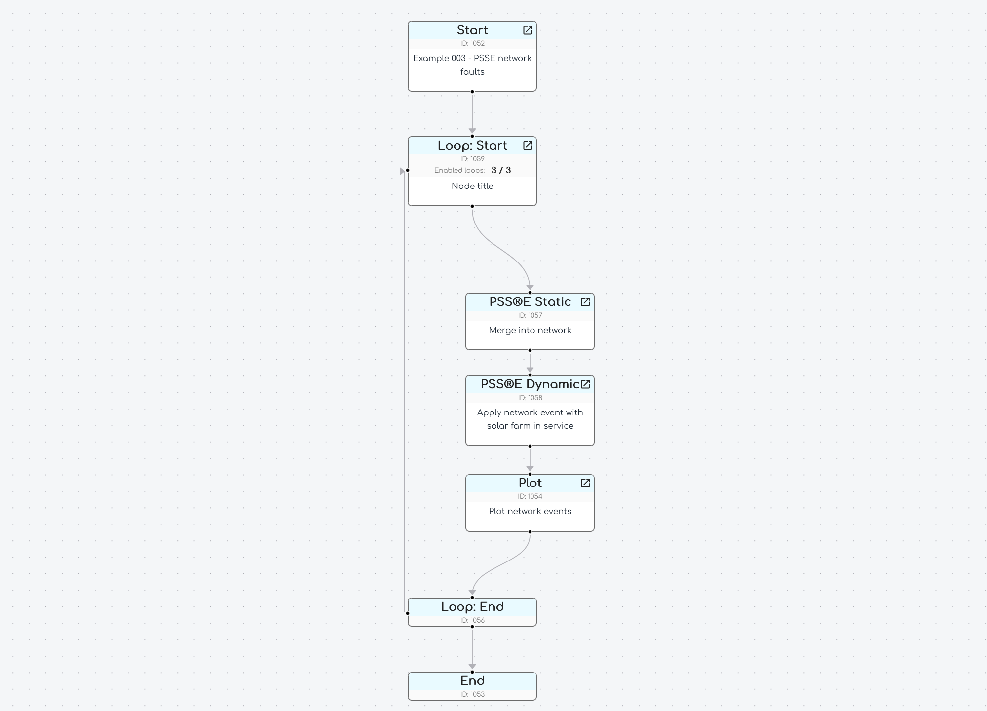
1) Start a new gridmo Project and add the following Nodes

• Start Node
• Loop Start Node
• PSS®E Static Node
• PSS®E Dynamic Node
• Plot Node
• Loop End Node
• End Node

Connect the Nodes so they appear as follows:

2) Set up auto-merge for the PSS®E Static Node

• Double click on the PSS®E Static Node to open the configuration window.
• Set the Model to gridmo\wecc-solar\psse\solar.sav to use an example 175 MW solar farm's PSS®E case file.
• Select the Define simulation & Define outputs tab.
  • In the Customize grid field select Merge into network
  • Set the Network model field to gridmo\distnet\distnetworkexample.sav to use an example network model with several pre-configured generators.
  • To merge bus number 1000 in the SMIB model with bus number 34502 in the network model, set:
    • The Model: Bus number field to 1000
    • The Network model: Bus number field to 34502
• Under the Commands field, add the following Commands:

PSS®E Static Node's Commands field

// Set POC P and V - then apply all CONTROL Commands at the same time
CONTROL, GEN=91003#S1, ATLINE=1001->1000#1, P=175
CONTROL, GEN=91003#S1, ATLINE=1001->1000#1, Q=FIXED, QTARGET=0
SOLVE
// No need to set SCR or XR as we are merging into a network case, and POC V is dictated by the network model

• The above Commands control our example solar farm to achieve P=175 MW, Q=0 MVAr at the solar farm's connection point after it has been merged into the network model.

3) Create Loop Variables in the Loop Start Node

• We are going to apply a series of network faults which we want to loop over. We could create multiple PSS®E Static and PSS®E Dynamic Nodes - however it is easier to use a Loop Start Node.
• Double click on the Loop Start Node to open the configuration window.
• Click the + button (far right hand side) to add a new Loop Variable.
• Add a Loop Variable called l_event_description and a second Loop Variable called l_event
  tip

  The l_ is optional, but recommended, as it'll help you remember that these are Loop Variables.

• Delete the existing example Loop Variable called l_new_variable_1 using the trash can icon next to its name.
• Delete the empty rows using the trash can icon next to the empty row, leaving one empty row.
• Click Apply (we will add events one at a time once we are all set up).

4) Configure the PSS®E Dynamic Node

• Double click on the PSS®E Dynamic Node to open the configuration window.
• Select the tickbox to enable Use model from linked PSS®E Static Node
• Set the Dynamics model data to gridmo\wecc-solar\psse\solar.dyr to use an example 175 MW solar farm's PSS®E dynamic data record.
• Select the Define simulation tab.
  • In the Customize grid field select Merge into network
  • Set the Network dynamics model data to gridmo\distnet\distnet_dyr.dyr to load the dynamic data records for all the generators in the example network model.
• Under the Commands field, add the following Commands:

PSS®E Dynamic Node's Actions field

// Put solar farm in V control mode (see PSSE Model PDF docs for ICON reference)
CONTROL, AT=0, ICON=M+5, GEN=91003#S1, DYRMODEL=REPCA1, VAL=1
// Set initial P at POC
CONTROL, AT=0, VAR=L+3, GEN=91003#S1, DYRMODEL=REPCA1, VAL=1, VALSCALE=0.875
// Apply the network event defined in the Loop Variable
$l_event

• The above Commands:
  • Put the solar farm in voltage control mode
  • Set the initial active power at the point of connection (POC) to 175 MW .
  • Apply the network event defined in the Loop Variable l_event.
• In the Define outputs tab, set theOutputs field to the following:

PSS®E Dynamic Node's Output field

// Values from our generator
OUTPUT, BUS=1000, VAL=V, NAME=i_ch_poc_v
OUTPUT, LINE=1001->1000#1, VAL=P, NAME=i_ch_poc_p
OUTPUT, LINE=1001->1000#1, VAL=Q, NAME=i_ch_poc_q
OUTPUT, BUS=91003, VAL=V, NAME=i_ch_terminal_v

// Values from network
OUTPUT, BUS=34501, VAL=V, NAME=i_ch_v_34501
OUTPUT, BUS=34502, VAL=V, NAME=i_ch_v_34502

• The above Commands output:
  • V, P and Q at our generators connection point.
  • V and two ends of a line we will apply the complex faults on.

5) Configure the Plot Node

• Double click on the Plot Node to open the configuration window.
• Set the Plot type to PDF to output a PDF file.
• Enter an output file name, such as Applying complex network events.
• Enter a plot title, such as Applying complex network events.
• For the plot subtitle, enter $l_event_description to display the description of the network event being applied as defined in the l_event_description Loop Variable.
• In the Define Subplots tab:
  • Set the x-axis minimum 0 and maximum to 20
  • Under Subplots select 1 page, 3 rows and 2 columns.
  • Click on the + to add a new subplot. For each subplot:
    • Enter a title in Subplot title, such as V at ABC 345 kV (Bus #34501) etc.
    • Under y-axis Channels enter each of the Internode Variables with the double curly brackets, such as {{i_ch_poc_v}}
  • Add 6 subplots in total (or as many as you wish to investigate) entering the Internode Variable reference from the PSS®E Dynamic node above.

We now have our gridmo project set up to apply complex network events.

Advanced examples

The following are additional examples covering a variety of different network events/faults/

Simulating a line fault without auto-reclose

We want to simulate the following event in our dynamic study:

• There is a fault on the line between PSS®E bus 34501 and 34502.
• The fault is very close to bus 34501 (10% of the line length from bus 34501).
• The fault is a three-phase fault.
• The line is disconnected by a protection relay at the bus 34501 end after 80 ms.
• The line is disconnected by a protection relay at the bus 34502 end after 220 ms.
• The line is out of service then for the rest of the simulation. No auto-reclose is attempted.

To implement this event:

• Double click on the Loop Start Node to open the configuration window.
• In the empty row under l_event_description enter (or add another row using the + Add Loop button):

Add the following to the Loop Start Node's 'l_event_description' field

Bolted 3PH fault 10% from ABC on ABC to XYZ No.1 345 kV line (Near 80 ms, far 220 ms, line out after fault).

• In the empty row under l_event enter:

Add the following to the Loop Start Node's 'l_event ' field

ADVFAULT, AT=5, TYPE=3PH, LINE=34501->34502#1, DURATION1=80, DURATION2=220, DISTANCE%=10

You can then launch the simulation (making sure the checkbox next to your new row in the Loop Start Node is ticked) and review the results:

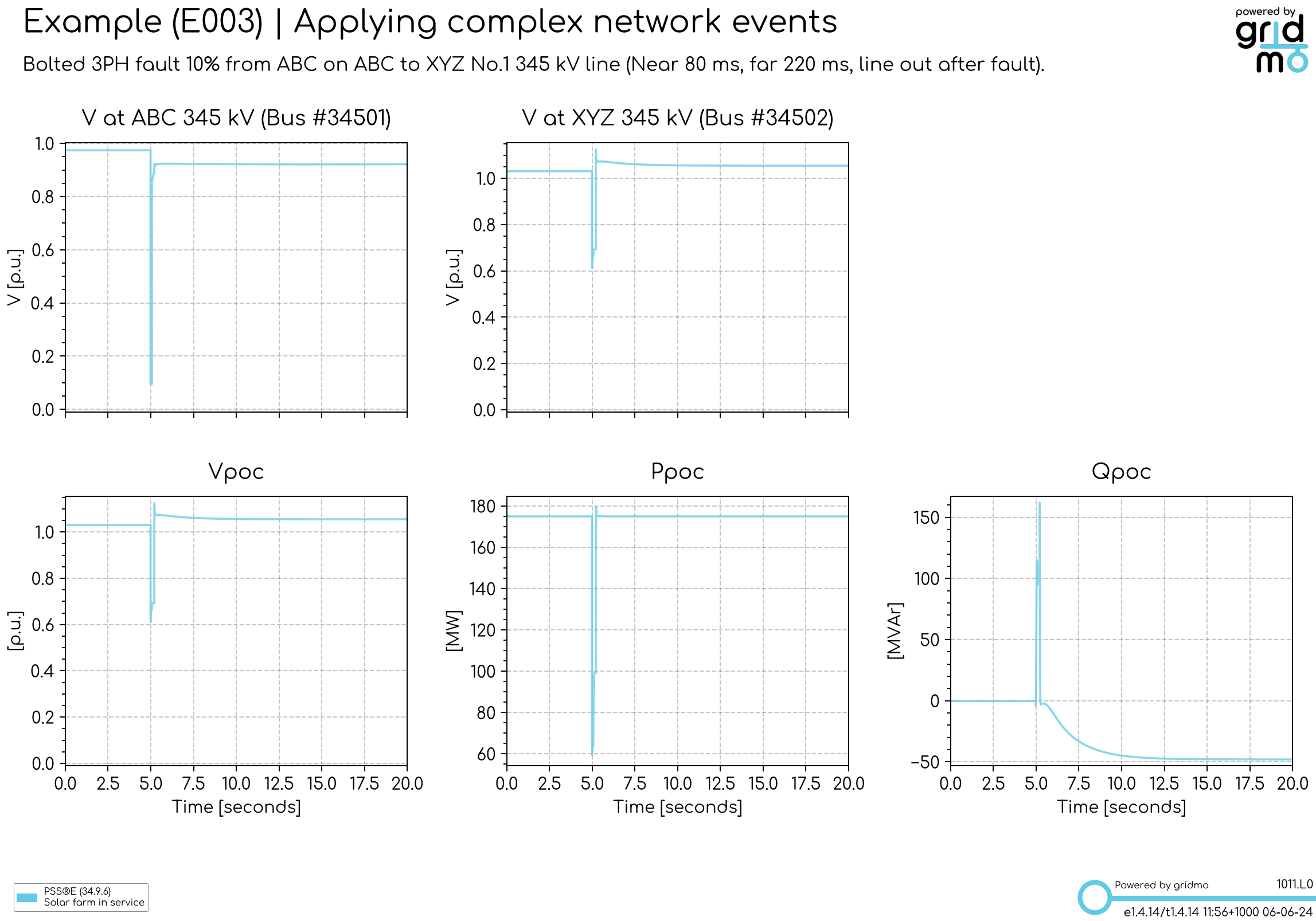
In the above plot, we can see the following:

• The voltage at both ends of the line is affected by the fault.
• The voltage dips to lower at the bus 34501 end of the line, as the fault is closer to this bus.
• The fault is cleared quicker from the bus 34501 end of the line than the bus 34502 end of the line as expected.
• The line is out of service for the rest of the simulation (we can tell that by the change in the voltage profile at the bus 34501 and 34502 ends of the line).

Simulating a line fault with auto-reclose

For our second event, we want the same line fault except now the line auto-recloses sucessfully after 3 seconds.

To implement this event:

• Double click on the Loop Start Node to open the configuration window.
• In the empty row under l_event_description enter (or add another row using the + Add Loop button):

Add the following to the Loop Start Node's 'l_event_description' field

Bolted 3PH fault 10% from ABC on ABC to XYZ No.1 345 kV line (Near 80 ms, far 220 ms, line recloses after 3 sec).

• In the empty row under l_event enter:

Add the following to the Loop Start Node's 'l_event ' field

ADVFAULT, AT=5, TYPE=3PH, LINE=34501->34502#1, DURATION1=80, DURATION2=220, DISTANCE%=10, AR_RETRIES=1, AR_FINALSTATE=IN, AR_DEADTIME=3000

The difference between this Command and the one previously is the addition of the auto-reclose optional arguments: AR_RETRIES=1, AR_FINALSTATE=IN, AR_DEADTIME=3000 - meaning retry once, after all retries the line is in service and with a dead time of 3 seconds (3000 milliseconds).

tip

gridmo by default implements auto-reclose logic assuming the tobus (which is 34502 in our example) has dead-line blocking enabled. That is, only the frombus end of the line will attempt to auto-reclose and only if its a successful auto-reclose, the tobus end will close.

This is to mimic the typical configuration of protection relays (to prevent unnecessary reclose attempts on a line which has a fault).

However - this performance is customisable, see the ADVFAULT Command

You can then launch the simulation (making sure the checkbox next to your new row in the Loop Start Node is ticked) and review the results:

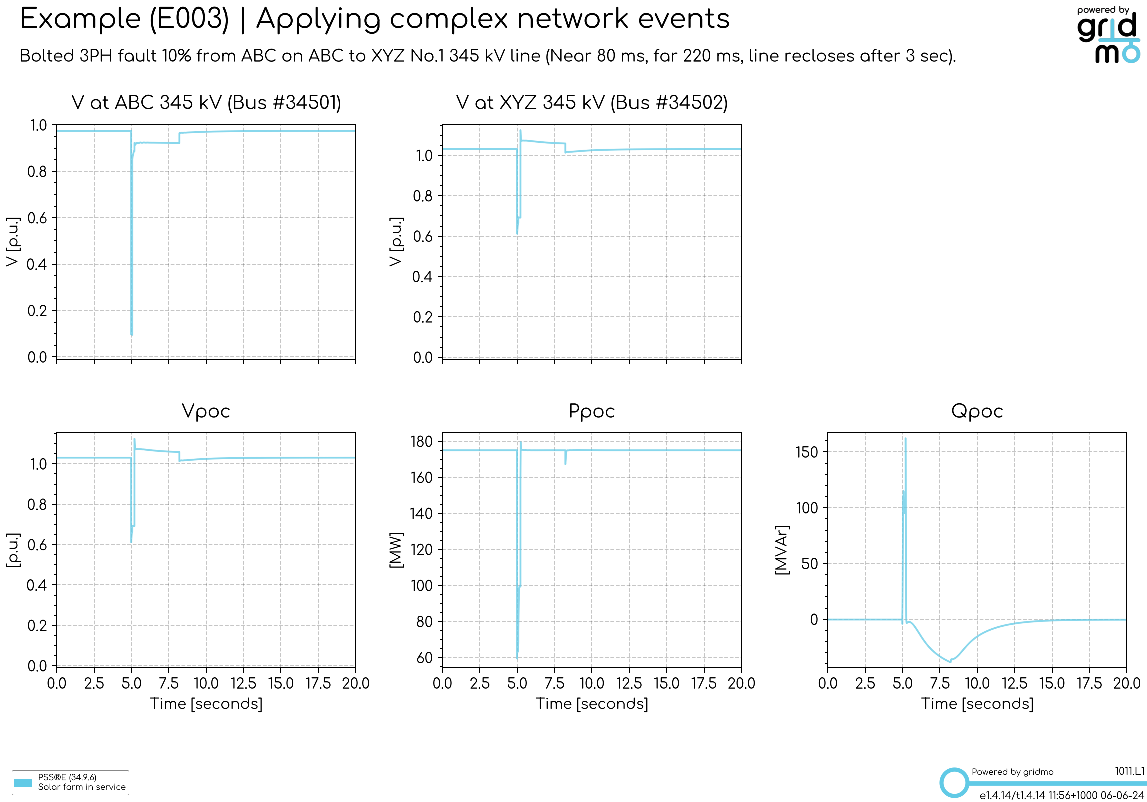
In the above plot, we can see the following:

• The line switches back in service at approximately 8 seconds in the simulation.
• We can see our solar farm ramping back to its pre-disturbance reactive power once the line is reclosed.

Simulating a line control trip

Now we want simulate a control trip, the sudden disconnection of a line without a fault present. Specifically we want:

• The line from bus 34501 to 34502 to be disconnected by a control room operator after 5 seconds in the simulation. No fault is present.

To implement this event:

• Double click on the Loop Start Node to open the configuration window.
• In the empty row under l_event_description enter (or add another row using the + Add Loop button):

Add the following to the Loop Start Node's 'l_event_description' field

Control trip of ABC to XYZ No.1 345 kV line (line disconnects without fault).

• In the empty row under l_event enter:

Add the following to the Loop Start Node's 'l_event ' field

SET, AT=5, LINE=34501->34502#1, STATUS=OUT

You can then launch the simulation (making sure the checkbox next to your new row in the Loop Start Node is ticked) and review the results:

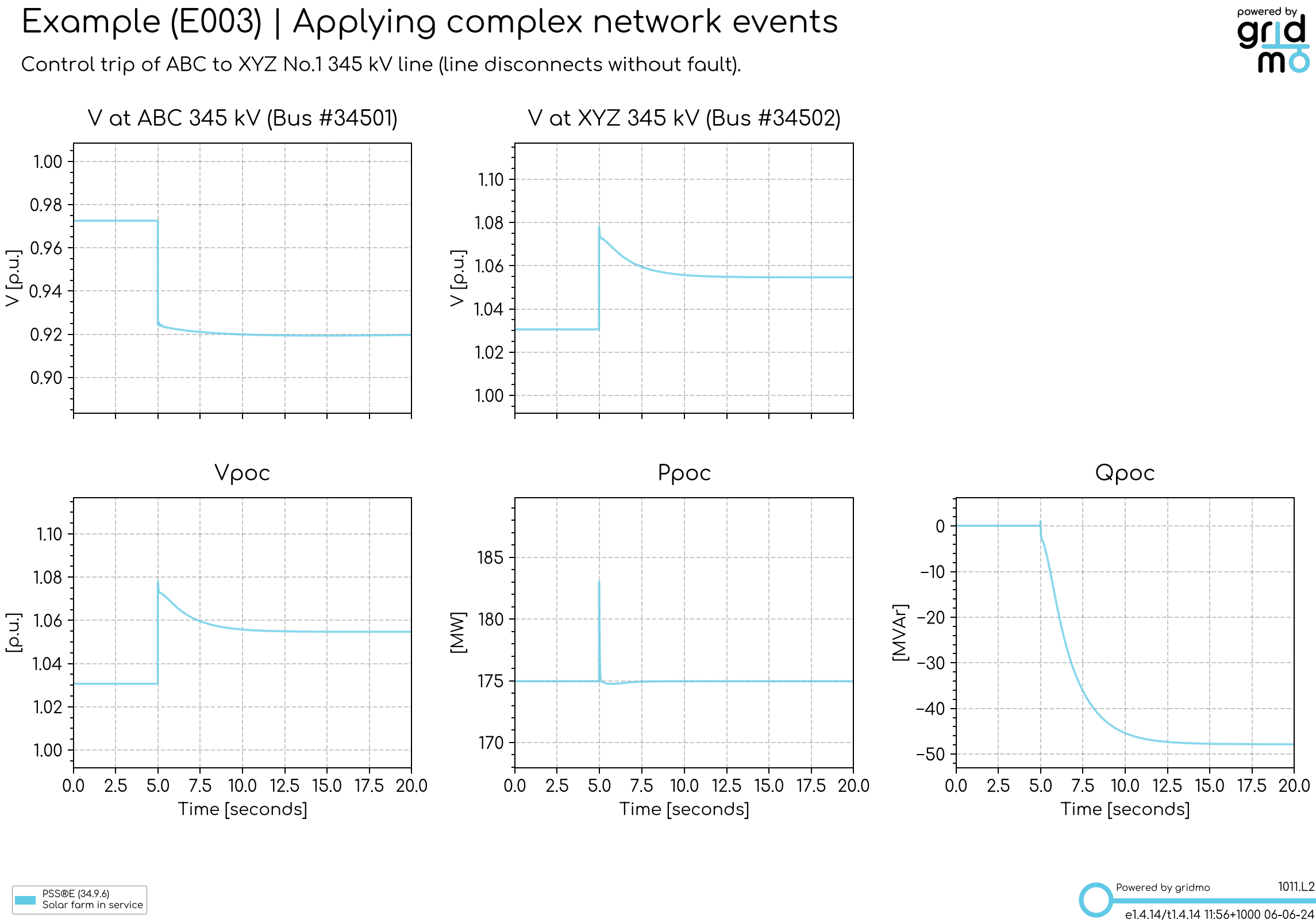
In the above plot, we can see the following:

• The line switches out at 5 seconds (we can see a difference in the voltages of bus 34501 and 34052).
• We can see our solar farm responding to the change in network conditions by changing its reactive power output.

Simulating a run-back scheme triggered by a line control trip

Now we want simulate a run-back scheme, the disconnection of a line which triggers a generator to run-back its active power to 0 MW. Specifically:

• The line from bus 34501 to 34502 is disconnected at 5 seconds in the simulation. No fault is present.
• The solar farm is instructed to run-back its active power to 0 MW after a delay of 2 seconds.

To implement this event:

• Double click on the Loop Start Node to open the configuration window.
• In the empty row under l_event_description enter (or add another row using the + Add Loop button):

Add the following to the Loop Start Node's 'l_event_description' field

Control trip of ABC to XYZ No.1 345 kV line (line disconnects without fault, triggers run-back after 2 sec).

• In the empty row under l_event enter (use Shift+Enter to add multiple lines)

Add the following to the Loop Start Node's 'l_event ' field

SET, AT=5, LINE=34501->34502#1, STATUS=OUT
CONTROL, AT=7, VAR=L+3, GEN=91003#S1, DYRMODEL=REPCA1, VAL=0 // run-back our solar farm to 0 MW

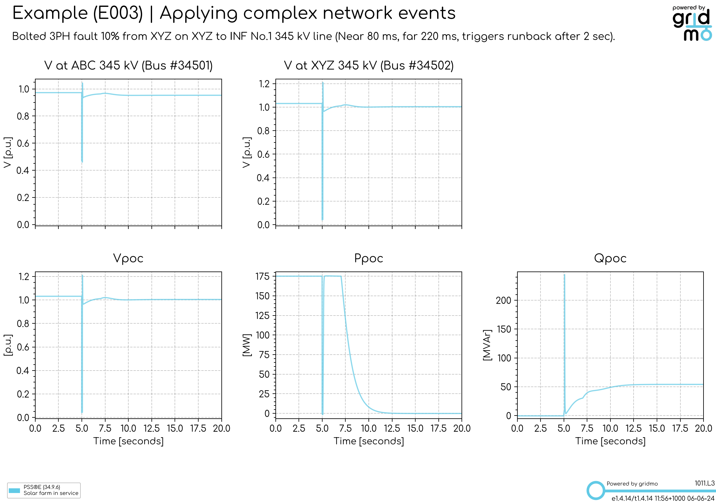
In the above plot, we can see the following:

• The line switches out at 5 seconds (we can see a difference in the voltages of bus 34501 and 34052).
• The solar farm reacts immediately to the change in network conditions by ramping its reactive power.
• 2 seconds after the fault, the solar farm ramps its active power output to 0 MW as per the run-back scheme.

Simulating an intertrip scheme

Now we want to simulate an intertrip scheme, the disconnection of a line which triggers a generator to immediately disconnect from the network. Specifically:

• The line from bus 34501 to 34502 is disconnected at 5 seconds in the simulation. No fault is present.
• The solar farm is instructed to immediately disconnect from the network after the line is disconnected.

To implement this event:

• Double click on the Loop Start Node to open the configuration window.
• In the empty row under l_event_description enter (or add another row using the + Add Loop button):

Add the following to the Loop Start Node's 'l_event_description' field

Control trip of ABC to XYZ No.1 345 kV line (line disconnects without fault, triggers intertrip).

• In the empty row under l_event enter (use Shift+Enter to add multiple lines)

Add the following to the Loop Start Node's 'l_event ' field

SET, AT=5, LINE=34501->34502#1, STATUS=OUT
SET, AT=5.42, GEN=91003#S1, STATUS=OUT

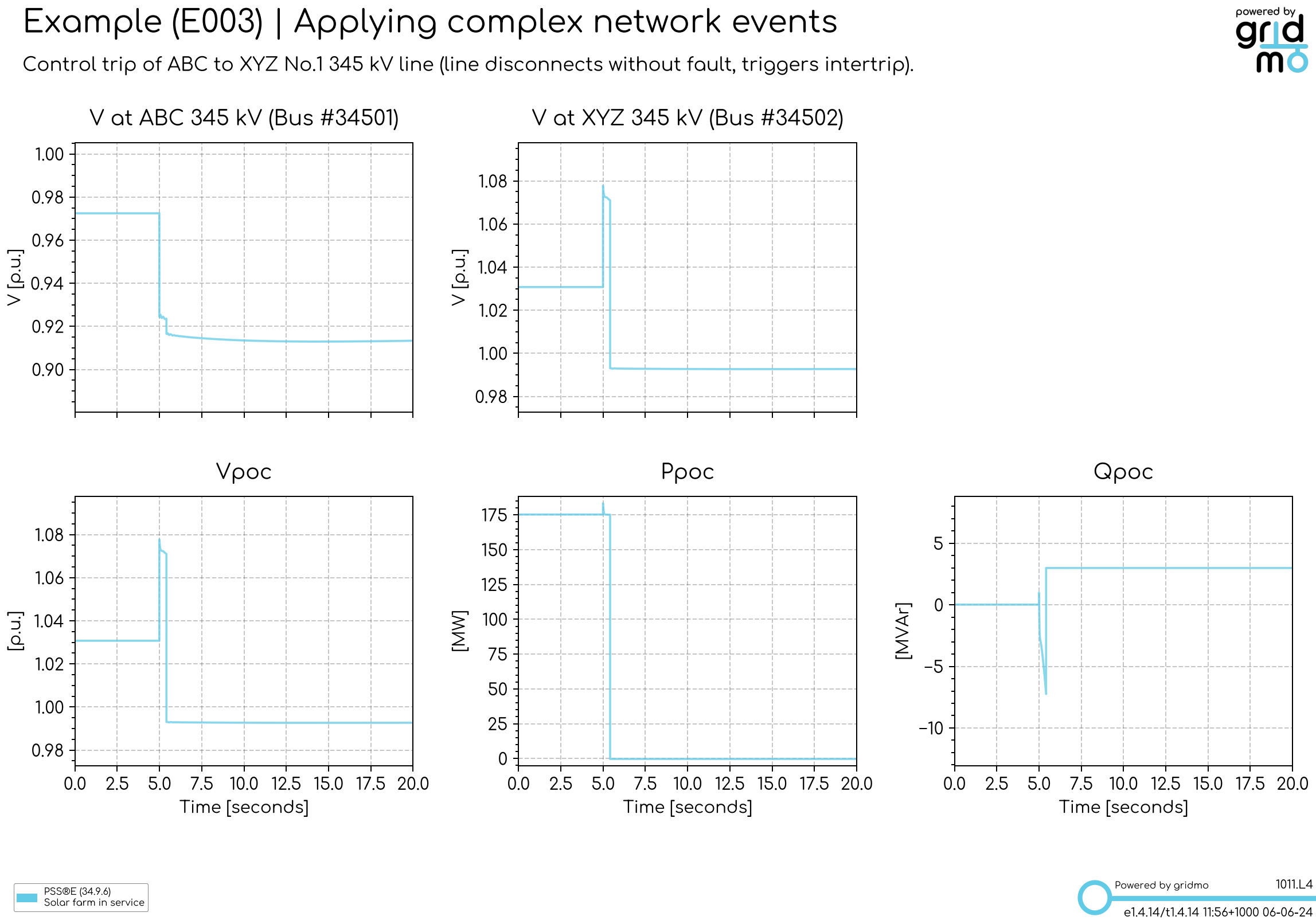
In the above plot, we can see the following:

• The line switches out at 5 seconds (we can see a difference in the voltages of bus 34501 and 34052).
• The solar farm disconnects at the end of the fault (point of connection P drops to 0 MW immediately).